Modeling Earth's Climate System with STELLA
Introduction to the Global Climate System
Insolation: Incoming Solar Radiation
Heat Transport by Evaporation and Condensation
Constructing a STELLA Model of the Climate System
1. Altering the Solar Input: Investigating the Response Time and Sensitivity
5. Comparing Different Causes of Warming
A More Advanced Model -- 3-Boxes
Introduction to the Global
Climate System
The Earth's climate system is an elaborate type of energy flow system (Fig.
1) in which solar energy enters the system, is absorbed, reflected, stored,
transformed, put to work, and released back into outer space. The balance
between the incoming energy and the outgoing energy determines whether the
planet becomes cooler, warmer, or stays the same. The Earth reflects about 34%
of the solar energy received; the remainder is used to operate the climate and
maintain the temperature of our planet. The Earth also radiates energy back
into space -- equivalent to 66% of the energy that is received -- this implies
that there is no net energy gain. Since the amount of energy received
approximately equals the amount given back to space, the Earth is approximately
in a steady state in terms of energy. As suggested in Fig. 1, this kind of a
steady state is an expected outcome of a system in which the outflow is
dependent on the amount of energy stored in the system. In reality, there are
temporal and spatial changes in temperature that are very important; some are
natural, while others may be due to anthropogenic modifications of the climate
system.
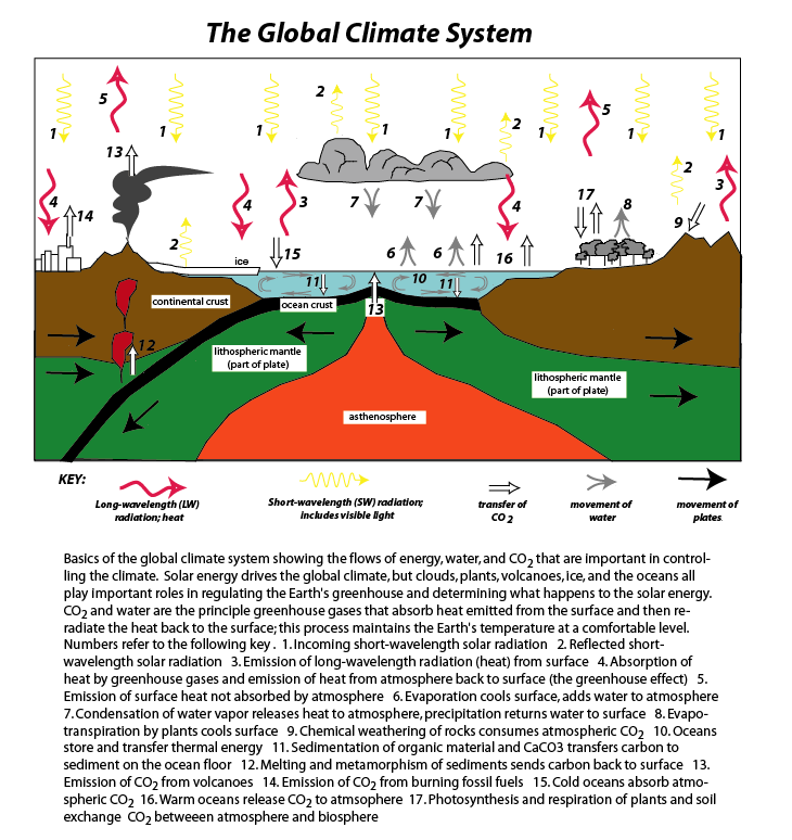
As shown in Figure 2 below, this system has important links with the global carbon cycle and the global hydrologic cycle; it also depends on the distribution of land masses and mountains and oceans over the surface of the Earth. Thus, a complete model of the climate system would have to include the dynamics of these other systems -- the result would be an enormously complex system, far beyond what is appropriate for a starting model. In making our model, we will focus on just the energy flows.
Before constructing a STELLA model of the Earth's climate system, we need to
study the details of how the solar energy is put to use, transformed,
transferred, stored, and released. Figure 3 shows a schematic diagram of the
energy flow for the Earth that illustrates what happens to all the energy we
receive. Some of the major features of this model are described briefly below.
Insolation -- Incoming Solar Radiation
Hydrogen fusion in the Sun creates an immense amount of energy, heating the
surface to around 6000°K; the sun then radiates energy outwards in the form of
ultraviolet and visible light. To simplify matters, we'll say that the total
amount of solar energy received by the Earth is equal to 100 units -- think of
this as 100% of the actual total, which is a rather unwieldy number (55.6 x
1023 Joules/year). To help put this number in perspective, it represents about
10,000 times the amount of energy generated and consumed by humans each year.
Another useful way to think of this comes from considering that the solar input
amounts to 343 Watts/m2 of Earth's surface. This is a bit less than
six 60 Watt light bulbs shining on every square meter of the surface, which
adds up to a lot of light bulbs since the total surface area of Earth is 5.1E14
m2.
Of the incoming 100 units of solar energy (see Fig. 3), 28 are immediately
reflected by clouds and 6 are reflected back from the land surface. Since it is
estimated that clouds presently cover about 60% of the surface of the Earth
[NASA, ERBE], we see that couds are not perfect reflectors -- they appear to
reflect about 47% of the solar energy. In contrast, the Earth's surface
(dominated by water) reflects about 7% of the incident solar energy. The
fraction of light that is reflected by a material is called the albedo. Black
materials have an albedo of 0 (no reflection) if they are perfectly black and
perfectly white materials have an albedo of 1.0 (total reflection). The table
below lists some representative albedos for a variety of materials that cover
the surface. Most of these albedos are sensitive to the angle of incidence of
the sunlight; this is especially true for water. When the Sun is at an angle of
40° and higher relative to the horizon, the albedo of the water is fairly
constant, but as the angle decreases from 40°, the albedo increases
dramatically, so that it is about 0.5 at a Sun angle of 10° and 1.0 at a sun
angle of 0°.
ALBEDO OF EARTH MATERIALS
Substance Albedo (% reflectance)
Whole Planet 0.31
Cumulonimbus clouds 0.9
Stratocumulus clouds 0.6
Cirrus clouds 0.5
Water 0.06 - 0.1
Ice & Fresh Snow 0.9
Sand 0.35
Grass lands 0.18 - 0.25
Deciduous forest 0.15 - 0.18
Coniferous forest 0.09 - 0.15
Rain forest 0.07 - 0.15
Most people have an intuitive sense of the affects of albedo on reflectance
and solar energy absorption. This is why people wear white clothes in hot sunny
climates and dark clothes in cold sunny climates. Applying the principle that
good absorbers are good emitters, you might choose to wear white clothes when
it is cold and cloudy.
As mentioned above, a total of 32 units of solar energy are reflected by our
planet; the remaining 68 units are absorbed. As shown in Figure 3, gases in the
atmosphere absorb 18 of these units, while the land surface absorbs 50 units,
with most of that being absorbed by the oceans. The absorption of solar radiation
in the atmosphere is due to water vapor, oxygen, ozone, and dust particles, all
of which can absorb energy within the ultraviolet-visible portion of the
spectrum. Materials on the surface -- rocks, plants, liquid water -- also
absorb in this part of the spectrum. Earth and atmospheric materials are also
capable of absorbing energy in the infrared part of the spectrum, which is the
energy emitted by the Earth surface and atmosphere. This infrared energy is
absorbed in the atmosphere by water vapor, carbon dioxide, and other gases such
as methane and CFCs.
As the atmosphere and Earth surface materials absorb ultraviolet, visible
light, or infrared energy, they gain thermal energy and their temperatures
rise. But, the rate of temperature rise with increasing thermal energy differs
for many materials -- this relationship is described by what is called the heat
capacity of a substance. The heat capacities for some common materials are
given in the table below.
HEAT CAPACITY OF EARTH MATERIALS
Substance Heat Capacity (Jkg-1K-1)
Water 4184
Ice 2008
Average Rock 2000
Wet Sand (20% water) 1500
Snow 878
Dry Sand 840
Vegetated Land 830
Air 700
The vast range of heat capacities is extremely important to the operation of
our climate system, and in particular, we should note the very high heat
capacity of water -- it heats up slowly, cools slowly, and retains heat better
than any other common substance. Heat capacities are also important when it
comes to figuring out how much thermal energy is stored in a given reservoir.
For instance, if we know the mass of a material and its heat capacity and its
temperature, we can calculate how much thermal energy is stored in the
material.
Equally important is the rate of heating that can be seen from the above
heat capacities. This information tells us that soil (some combination of wet
and dry sand and vegetation gives a heat capacity of around 1000) warms up
about 4 times faster than water, given the same rate of energy input, and air
warms up somewhat faster than soil. Actually, the rate of warming is a bit more
complex than just comparing heat capacities because the rate of energy input
depends the albedo.
All objects whose temperatures are above absolute zero emit energy
proportional to their temperature. This energy is emitted in the form of
electromagnetic radiation whose average wavelength is inversely proportional to
the object's temperature. The rate of energy given off through radiation by an
object is proportional to the fourth power of the object's temperature and is
described in the following equation:
F = esAT4
where F is the rate of energy flow in Joules/sec (or Watts), e is the
emissivity of the object, s
is the Stefan-Boltzmann constant, A is the surface area of the object, and T is
the temperature of the object in degrees Kelvin. The Stefan-Boltzmann constant
has a value of 5.67E-8 Joules/sec m2 K4. The emissivity
is a dimensionless number and ranges from 0 to 1; a perfect black body has an
emissivity of 1, while very shiny objects have an emissivity of close to 0.
Human skin has an emissivity of 0.6 to 0.8. For the purposes of our simple
model, the important thing is that the energy emitted is proportional to the
fourth power of the temperature.
Given the range of temperatures on Earth's surface, this emitted radiation
occurs mainly within the infrared part of the spectrum. Earth's surface emits
106 units of energy as infrared radiation; of this, 99 units are absorbed by
greenhouse gases in the atmosphere, with the remaining 8 units pass through the
atmosphere (this "leak of 8 units is a measure of the efficiency of
Earth's greenhouse). The atmosphere also emits infrared energy -- 79 are
directed back to the Earth's surface, while 58 are directed to outer space .
The 79 units sent back to the surface are absorbed and then re-radiated to the
atmosphere, which again absorbs most of it and then returns much of that back
to the surface, recycling the energy and giving rise to the famous greenhouse
effect.
Heat Transport by Evaporation and Condensation
Earth's surface also contributes heat to the atmosphere in two other ways.
30 units of energy are transferred to the atmosphere by the evaporation of
water at the surface and the later condensation of that water vapor in the
atmosphere. When water evaporates, it steals heat from the surface; that heat
is called latent heat and is released when the vapor condenses.
Air in direct contact with the surface is heated and then rises,
transporting that heat to higher levels in the atmosphere -- this process of
convection transfers 6 units of energy from the surface to the atmosphere.
The climate system of the Earth is thus a set of related processes that
transfer and transform energy, storing it and putting it to work, and in the
process, determining the temperature of our planet. This dynamic system is
therefore an energy flow system rather than a material flow system; it is also
an open system since we are not concerning ourselves with the ultimate sources
and sinks of this energy.
Constructing a STELLA Model of the Climate
System
In moving from the conceptual model to a working computer model, we need to
identify the major reservoirs and flows that will constitute the model. In this
case, we can study Figure 3 and see that there are naturally 2 major reservoirs
-- the atmosphere and the Earth's surface. There are numerous flows, but here,
we will combine some of them to increase simplicity, arriving at six flows.
These flows and reservoirs can be seen in a STELLA diagram of the system shown
in Figure 4.
Download
pre-made models for use in PSU Geoscience 001 lab
Initial Values of Reservoirs
To create a model of this energy system, we need to know the starting
amounts of thermal energy in the various reservoirs. This model will have just
two reservoirs where energy is stored -- the atmosphere and the Earth's
surface, which includes the oceans and the soil. Here, I've assumed that the
oceans cover 70% of the surface (an area of about 3.57E14 m2) and
about 35 meters of water is actively involved in the heat exchange with the
surface on a time scale of a few years. This allows us to calculate the total
mass of water (using a density of 1000 kg/m3), and then if we assume an average
temperature of 15°C (or 288°K) and a heat capacity from the table above, we get
the total energy stored in the oceanic part of the reservoir. This number,
1.5E25 Joules, is about 2.7 times greater than the total amount of energy
received by the Earth from the Sun in one year -- or 270 of our energy units
because we've said that 100 units is equal to the total annual solar energy
received. Going through the same calculations for soil (land area is 1.53E14 m2),
assuming that only one meter of soil or rock is involved, using a density of
1500 kg/m3 and a heat capacity of 1000 J/kg°K, we end up with 6.6E22 Joules, a
measly 1.2 units of energy. So the Earth Surface reservoir will be given an
initial value of 271.2 units. We do the same calculation for the atmosphere,
assuming a mass of 5.14E18 kg, an average temperature of -18°C, and a heat
capacity of 700 J/kg°K, which results in 9.17E23 Joules, or 16.5 units of
energy for the Atmosphere reservoir.
Definition of Flows
The next step is to decide how these flows will be mathematically defined --
will they be constants or equations with variables? Below, I briefly describe
how each flow is defined.
Solar to Surface
This is the solar energy that reaches and is absorbed by the land surface,
which is strongly dependent on the percentage of the surface covered by clouds,
but also on the albedo of the surface, and the portion of the insolation that
is absorbed by the atmosphere. A simple formulation for this is:
Solar_to_Surface = (Solar_Input-Reflected_Insolation)*(1-SW_Atmos_Absorp)*
(1-Surface_Albedo)
Solar_Input will start with a constant value of 100 units/year (it will be
altered in subsequent experiments). Reflected_Insolation is the solar radiation
reflected back into space by clouds and is defined as:
Reflected_Insolation = Solar_Input*Cloud_cover*Cloud_Albedo
Cloud_cover is the fraction of the Earth's surface covered by clouds,
initially set at 0.60, equivalent to 60%. Cloud_Albedo is set at 28/60, close
to 0.5. The fraction is used here to make the equations yield whole numbers.
SW_Atmos_Absorp is the fraction of solar insolation that is absorbed by the
atmosphere, estimated to be 0.25 or 25%. Surface_Albedo is the average albedo
of the surface (dominated by water in the oceans) and is entered as 4/54, a bit
less than 0.1.
The result of these calculations is that 50 units of energy are absorbed by
the surface.
Solar to Atmosphere
This flow is defined using the same approach as the Solar to Surface flow:
Solar_to_Atmos = SW_Atmos_Absorp*(Solar_Input-Reflected_Insolation)
The terms in this equation are defined as described above, and the result of
the calculations is that 18 units of energy are absorbed by the atmosphere.
Surface LW Loss
Some portion of the infrared radiation emitted from the surface escapes,
passing through the atmosphere without being absorbed -- this is energy lost
from the system. The magnitude of this flow is currently estimated to be 8
units of energy, but it is also a function of the temperature (specifically the
fourth power of the temperature) of the surface since the temperature determines
the overall amount of infrared energy emitted. A simple way of expressing this
is:
Surface_LW_to_space = 8*((Surface_Temp/288)^4)
Here, 288 is the starting temperature in °K of the Earth's surface (15°C)
and Surface_Temp is the temperature in °K at any time during the model run.
Atmosphere LW Loss
Analogous to the previous flow, this one is designed to change as the
temperature of the atmosphere changes:
Atmos_LW_loss = 60*((Atmos_Temp/255)^4)
The starting temperature of the atmosphere is here set at 255°K or -18°C.
Surface to Atmosphere
This flow is a conglomeration of several different processes -- emission of
infrared energy (116 units), heat transfer through evaporation and
condensation, and convective motion of air that is warmed at the surface (36
units). A full mathematical formulation of these three processes would be far
too complex for a model of this sort, so we will instead apply the simple
assumption that all of these processes will depend on the temperature of the
Earth surface in a relatively simple fashion:
Surface_heat_to_atmos = (108*((Surface_Temp/288)^4))+(36*Surface_Temp/288)
As discussed above, the ssion of infrared energy is proportional tot eh
fourth power of the temperature, and we'll assume that the other processes
follow a more basic linear relationship with the temperature. In this linear
relationship, if the surface temperature doubles, then the heat flow also
doubles.
Atmosphere LW to Surface
This flow represents the emission of infrared energy from the atmosphere
back to the surface -- the greenhouse effect. The magnitude of this flow is
really just a function of the temperature of the atmosphere (which in turn is a
function of how much infrared energy is absorbs), and so we define the flow
with a non-linear (fourth power) temperature dependence like the other flows
that represent radiative heat transport:
atmos_LW_to_surface = 102*((Atmos_Temp/255)^4)
Summary of Model Equations
Below, all system components are summarized, printed in the same format used
by the program.
RESERVOIRS:
INIT ATMOSPHERE = 16.5 {% energy in Joules relative to total annual solar energy input}
INIT SURFACE = 271.2 {% energy in Joules relative to total annual solar energy input}
FLOWS:
Solar_to_Surface = (Solar_Input-Reflected_Insolation)*(1-SW_Atmos_Absorp)*(1-Surface_Albedo)
{solar energy absorbed by the surface}
Solar_to_Atmos = SW_Atmos_Absorp*(Solar_Input-Reflected_Insolation)
{SW Radiation received by the atmosphere}
Surface_heat_to_atmos = (108*((Surface_Temp/288)^4))+(36*Surface_Temp/288) {heat transferred to the atmosphere by radiation, condensation of water, and conduction-convection }
Atmos_LW_loss = 60*((Atmos_Temp/255)^4) {this is infrared energy -- heat -- that is radiated out into space}
Atmos_LWto_surface = 102*((Atmos_Temp/255)^4)
{heat -- infrared energy radiated down to the surface, aka the greenhouse effect}
Surface_LW_to_space = 8*((Surface_Temp/288)^4) {infrared heat loss -- the atmosphere doesn't
absorb all energy within the infrared; this is a function of the abundance of greenhouse gases}
CONVERTERS:
Atmos_del_T = Atmos_Temp-255 {°K -- atmos temp relative to starting temp}
Atmos_Temp = 255*ATMOSPHERE/16.5 {starting avg temp for atmosphere is 255°K = -18°C this relationship incorporates the avg. heat capacity of the atmosphere}
Cloud_Albedo = 28/60 {clouds reflect 50% of the incident solar SW radiation}
Cloud_cover = .6 {average fraction of globe covered by clouds}
Reflected_Insolation = Solar_Input*Cloud_cover*Cloud_Albedo
Solar_Input = 100
{100 units is the annual amount of solar energy received by Earth, equal to 55.6E23 Joules/year}
Surface_Albedo = 4/54 {% reflectance, set so that initially, 4 units are reflected back into space}
Surface_del_T = Surface_Temp-288 {°K -- surface temp relative to starting temp}
Surface_Temp = 288*SURFACE/271.2 {°K -- starting temp for surface is 288°K = 15°C}
SW_Atmos_Absorp = .25 {absorption of insolation -- UV and visible radiation -- in the atmosphere,
due to ozone, water, and dust }
Using the model structure as shown in Figure 4 along with these definitions
of the model components, you can create a working version of this climate
system model. Once the model is assembled and the components are defined, the
model should be in an initial steady state -- nothing should change. This
steady state serves as the control for a series of experiments in which
different aspects of the system are changed in order to answer specific
questions.
Because of the energy flow values chosen here -- 100 units is equal to the
amount of energy received by Earth each year -- the basic unit of time for the
model is one year. But, the calculations have to be done in shorter time steps
because of the magnitudes of the flows relative to the size of the atmosphere
reservoir. As a general rule of thumb, the time step, or DT of the numerical
integration that the program performs has to be small enough so that in each
calculation, the withdrawals from a reservoir do not exceed the amount in the
reservoir. As with all numerical integrations, the shorter the time step, the
better the solution -- the trade-off is that a shorter time step means more
calculations and thus slower performance. In the case of this model, a time
step of 0.01 gives good results (reducing the time step further does not alter
the results).
While performing experiments with this model, it may be especially helpful
to monitor changes by plotting the two converters called Surface_del_T and
Atm_del_T; these represent the change in the temperature of the reservoirs from
their initial values. But, you should feel free to plot any and all parameters
in teh model in order to better understand why the system behaves as it does.
For each of the experiments below, there are a few questions that you can
consider to help guide your inquiry. I do not include graphs of the results
here because I want to encourage you to make these models and run them and
think about them on your own.
1. Altering the Solar Input -- Investigating the Response
Time and Sensitivity
In this experiment, we investigate two simple questions: 1) How quickly does
our model climate system respond to changes (what is its response time)?; and
2) How sensitive is this climate system to changes in the solar energy received
by Earth? Restating question 2, if we change the solar input by 3%, how much warmer
does the our model Earth become and how quickly will it accomplish this
warming? Furthermore, we may ask what the pattern of response is -- which part
of the system reacts more quickly and which more slowly? We know that the solar
input does vary in the real world, so these are reasonable experiments to do.
We can begin to answer these two questions very simply, by changing the
value of the solar input in a stepwise fashion, observing the response by
plotting the Surface_del_T and Atmos_del_T converters. Using the Sensitivity
Specs window in STELLA, we can easily run a whole series of model simulations
with specified changes in the solar input.
The response time of the system as a whole is related to the lag time of the
system, which can be observed through another experiment in which we create a
spike in the solar input. To do this, we redefine the solar_input converter,
making it a graphical function of time (this procedure is clearly explained in
the STELLA manual; set Solar_Input equal to TIME, then click the Become Graph
button to define this graphical function) such that it begins at a value of
100, then jumps up to a value of 103, then immediately returns to 100.
- What are the lag times of the two reservoirs? Why is one shorter than another?
- Are the lag times a function of the length of time of the solar spike?
- Based on these experiments, what can you predict about the relationship between the winter solstice (minimum insolation in N. Hemisphere) and the coldest part of the year?
In this experiment, we ask what will happen if we change the percentage of
the surface covered by clouds. We can easily explore this question by first
increasing and then decreasing the percent cloud cover converter -- up to 65%
and then down to 55%. Before actually running the model, it is useful to make a
prediction about what will happen. As before, it is probably best to study the
changes in the temperatures of the two reservoirs using the Surface_del_T and
Atmos_del_T converters. Results are shown in Figure 6a and 6b.
Moving beyond this simple experiment, we next modify the way that cloud
cover is defined, making it dependent on the global temperature. The reasoning
here is that when the Earth is very cold, there will be less evaporation,
therefore less water vapor to form clouds in the atmosphere, and conversely,
when it is warmer, there will be a greater percentage of the Earth covered by
clouds. In reality, as the water content of the atmosphere changes, we would
have to change the part of the system that relates to the greenhouse efficiency
and the latent heat transport (through evaporation and condensation of water)
if we wanted a model that is as realistic as possible. But, we will ignore
these refinements in order to maintain the simplicity of the model.
To make the change, draw a connector arrow between the Surface_Temp
converter and Cloud_Cover converter; this will cause a question mark to appear,
signaling the need to redefine the converter. Double-click on Cloud_Cover and
set it equal to Surface_Temp and click on the Become Graph button; this will
place Surface_Temp along the x-axis. Set the lower range of the x-axis to 258
(the units here are °K) and the upper range to 318, giving you a range of 30°
on either side of the starting temperature. Make sure that the Data Points box
of this dialog window is set at 7, and then you will see that a temperature of
288 is one of the Input values; this will allow you to set the Cloud_Cover at
0.44 when the surface temperature is 288, thus preserving the initial
conditions of the model. Where do you go from here? There really aren't any
data we can turn to draw this graph properly, that is, in a way that mimics
what really happens on Earth; the main reason is that we have not observed the
global cloud cover over this whole range of temperatures. But, it is generally
believed that at lower temperatures, the cloud cover will decrease and at
higher temperatures, it will increase (Dickinson et al., 1996). This suggests
that the slope of the line ought to be positive, moving up to the right. For
the sake of simplicity, let's say that over this range of temperatures, the
cloud cover will vary according to the table below:
Input Output
258 0.015
268 0.110
278 0.360
288 0.600
298 0.840
308 0.920
318 0.950
Now the question is: How do we evaluate the effect of this change? If we
just run this model without making any additional changes, what will happen?
Since we've defined the graph such that the initial cloud cover will be 0.60,
and cloud cover can change only if the temperature of the Surface reservoir
changes, the system should be in a steady state, identical to the initial
model. This might lead to the false conclusion that this change had no effect
on the system. A more meaningful control in this case is the experiment where
we changed the Solar Input to 103, effectively turning up the heat. But before
running this modified model, make a prediction about what will happen.
- This new change represents a kind of feedback mechanism. Is it positive or negative?
- Explain why this model behaves as it does.
- How does this model differ in terms of performance with the original (the "control" model)?
Now we move on to a more severe modification, investigating the behavior of
our model upon removal of the greenhouse effect. As shown in Figure 2, the
greenhouse effect is represented by the absorption of 108 units of infrared
energy by the atmosphere and then the return of 102 units back to the land surface.
The 102 units returning are simply a result of the radiation of the atmosphere;
it will radiate heat back to the surface regardless of how or from where that
heat energy came from. So, in looking for the right way to dismantle the
greenhouse, we ought to leave the Atmos_LW_to_surface flow alone. Similarly,
the 58 units of energy leaving the atmosphere is just the rate of upward energy
loss from the atmosphere, so we'll leave that alone too. The simplest way to
remove the greenhouse effect is to remove the 108 units of energy emitted by
the land that is absorbed by the atmosphere in our original model. But, those
108 units can't just disappear; this energy has to go someplace else, and by
increasing the Surface_LW_to_space flow from 8 to 116, we can conserve the
energy in our system. We'll leave the Cloud_Cover defined as previously --
varying with the global temperature.
To make this modification, we need to change two flows --
Surface_heat_to_atmos and Surface_LW_to_space. The changed definitions of the
flows are summarized below:
Surface_LW_to_space = 116*((Surface_Temp/288)^4)
Surface_heat_to_atmos = (36*Surface_Temp/288).
Here, the original model serves as an appropriate control if we simply want
to understand what happens when we turn off the greenhouse. As always, it is
useful to make a prediction before running the model.
- Based on the results, how much of a warming effect does our greenhouse have?
We next explore the effect of enhancing the greenhouse, simulating what may
happen in the near future as we continue to burn more fossils fuels and clear
more forests, thus increasing the concentration of carbon dioxide in the
atmosphere. Our goal here is to model the effects of doubling atmospheric CO2
. At present, CO2 accounts for perhaps 30% of the total infrared
energy absorbed by the atmosphere, which would about 36 units of the 108 that
are absorbed by all greenhouse gases in the atmosphere. You might imagine then
that doubling CO2 would lead to an additional 36 units of energy
absorbed, but in fact, the relationship between the concentration of CO2
in the atmosphere and the absorption of heat is not linear -- at higher
concentrations, increases in CO2 produce less and less of an effect.
Calculations (Shine, et al., 1995) have shown that a doubling of CO2
is expected to increase the energy trapped by 4 W/m2, which is a bit
more than 1% of the Solar Input (343 W/m2), or 1.2 units in our
model here. So, to modify our model, we increase the infrared part of the
Surface_heat_to_atmos flow to 91.2 units and decrease the Surface_LW_to_space
flow to 6.8 units. The modified flows are thus:
Surface_LW_to_space = 6.8*((Surface_Temp/288)^4)
Surface_heat_to_atmos=109.2*((Surface_Temp/288)^4)+(36*Surface_Temp/288).
- How much warming does this produce? For reference, keep in mind that over the last 100 years, the global temperature appears to have increased by about 0.8°C while the concentration of atmospheric CO2 increased by about 20% (going from about 290 ppm to 350 ppm). In considering these results, it is interesting to note that published estimates of the global warming due to a doubling of CO2 , made using the most sophisticated climate models possible range from 1.5 to 4.5°C (Kattenberg et al., 1996).
5. Comparing Different Causes of Warming
Here, we consider the question of whether we can distinguish between warming
caused by an increase in the Solar Input vs. warming caused by an enhanced
greenhouse. This is related to the question of whether or not we can rule out
the possibility that the current warming observed for our planet is caused by a
slight increase in the solar input. It turns out that with a Solar Input value
of 102, you get virtually the same amount of warming of the land surface as you
do with the enhanced greenhouse that results from a doubling of CO2
. This experiment is easiest to analyze in the form of two separate models run
at the same time. To do this, copy and paste the existing model off to the side
of the initial model, then restore the greenhouse to the initial state in one
of the models and increase its Solar Input to 101.25, leaving the other model
with the enhanced greenhouse as described in experiment 4 above. Plot similar
elements of the two models on the same graphs to look for variance in these
models.
- After running these tandem models, can you distinguish between warming caused by an increase in the insolation vs. warming caused by an enhanced greenhouse? What kinds of data would you need to examine to be able to answer this question for the Earth?
Global measures of the temperature of the atmosphere are not too precise and
the record does not go back so far, so a direct test of this model result is
not easy. However, with a warmer atmosphere, the nightime low temperatures of
the surface should also be warmer. If this warming took place gradually, then
the daytime highs of the surface would also be increasing, but less rapidly
than the nightime lows. Another way of saying this is that the magnitude of the
daily surface temperature variation should be decreasing even as the whole
system is warming. In fact, Karl et al. (1993), and Mitchell et al. (1995) have
noticed that the night-time temperatures seem to be increasing more rapidly
than the daytime temperatures -- the diurnal temperature variations seem to be
decreasing. Of course, we must always be cautious in projecting the results and
implications of such a simple model, it is nevertheless important to realize
that the actual measurements are consistent with the hypothesis that the present
warming is caused primarily by an enhanced greenhouse rather than increased
solar energy.
Moving Forward:
A More Advanced Model -- 3-Boxes
References Cited
- Dickinson, R.E., Meleshko, V., Randall, D., Sarachik, E., Silva-Dias, P., and Slingo, A., 1996, Climate Processes, in Houghton, J.T., Meira Filho, L.G., Callander, B.A., Harris, N., Kattenberg, A., and Maskell, K., (eds.) Climate Change 1995, Cambridge University Press, Cambridge, 572 p.
- Shine, K.P., Fouquart, Y., Ramaswamy, V., Solomon, S., and Srinivasan, J., 1995, Radiative Forcing, in Houghton, J.T., Meira Filho, L.G., Callander, B.A., Harris, N., Kattenberg, A., and Maskell, K., (eds.) Climate Change 1994, Cambridge University Press, Cambridge, 572 p.
- Kattenberg, A., Giorgi, F., Grassl, H., Meehl, G.A., Mitchell, J.F.B., Stouffer, R.J., Tokioka, T., Weaver, A.J., and Wigley, T.M.L, 1996, Climate Models -- Projections of Future Climate, in Houghton, J.T., Meira Filho, L.G., Callander, B.A., Harris, N., Kattenberg, A., and Maskell, K., (eds.) Climate Change 1995, Cambridge University Press, Cambridge, 572 p.
- Karl, T.R., Knight, R.W., Kukla, G., Plummer, N., Razuvayev, V., Gallo, K.P., Lindseay, J., Charlson, R.J., and Peterson, T.C., 1993, Asymmetric trends of daily maximum and minimum temperature: Bulletin of the American Meteorological Society, v. 74, P. 1007-1023.
- Mitchell, J.F.B., Davis, R.A., Ingram, W.J., and Senior, C.A., 1995, On surface temperature, greenhouse gases and aerosols: models and observations: Journal of Climate, v. 8, p. 2364-2386.
- Strahler, A.N., and Strahler, A.H., 1989, Physical Geography, 4th Ed., New York, John Wiley and Sons, 562 p.
- Schneider, Coevolution of Climate and Life
- Henderson-Sellers, A. and McGuffie, K. A Climate Modelling Primer, Wiley, New York, 217p.
- Peixoto and Oort, Physics of Climate