Meteo 465
Middle atmospheric dynamics
You can augment your reading with Holton, Chapters 10 and 12.
While it is correct to state that the general atmospheric circulation is driven by the differential absorption of solar energy at the surface, this statement may be only partially correct for some regions, such as the stratosphere. For the stratosphere, eddies are as fundamental to the circulation as the differential solar heating.
In discussing the general circulation, we will be looking for those processes that maintain the mean zonal, and meridonal circulations. We will see that these are coupled and that waves have a lot to do with it.
Without eddies,
· the zonal mean temperature would match, with a ~10-20 day lag, the radiative equilibrium temperature and would vary annually;
· the flow would be only the zonal mean flow, which is determined by the meridional temperature gradient and the thermal wind balance;
· there would be no stratosphere troposphere exchange;
Heating and cooling patterns result from eddies driving the stratosphere away from radiative equilibrium.
Important quantities:
1. Potential temperature (units: K).
q = T (po/p)R/cp = T
(1000/p)0.286
Potential temperature is conserved when there are no diabatic effects. An air parcel will tend to move on an isentropic surface, or surface of constant potential temperature.
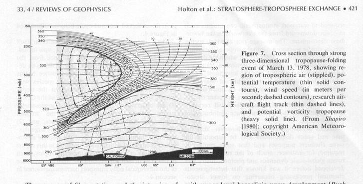
2. (Ertel’s) Potential vorticity (units: K kg-1 m2 s-1).
PV = (z + f) (-g ¶ q /¶p)
where z = k·(Ñ x u) is the relative vorticity, which can be either shear vorticity or curvature vorticity.
PV is conserved in an adiabatic, frictionless flow.
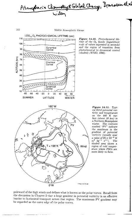
The figure give the PV in the stratosphere relative to the troposphere.
3. Geopotential height:
F = ò g dz
We need also consider geostrophic winds, which are the balance of Coriolis and pressure gradient forces.
vg = - (1/f) ¶ F/¶x
ug = - (1/f) ¶ F/¶y
where F = ò g dz, the geopotential height, R = gas constant, H = scale height, and f = 2W sinj ~ 10-4 s-1 @ 45oN, the Coreolis parameter.
In the analysis to follow, we will assume that the motions are approximately geostrophic, or quasi-geostrophic.
Now, ![]()
From these equations, we can derive the thermal wind equations:
 and
and 
where the “p” subscript implies that the differentiation occurs while the pressure is constant.
Let’s look at the zonal mean circulation first and then we will move on to the mean meridional circulation. We will use the log-pressure coordinate:
z = -H ln(p/po),
where po is taken to be 1000 hPa.
1. Start with the equations of motion:
conservation of momentum:
![]()
![]()
where the first term is the total
derivative of u and v, ![]() , the second term is the Coriolis forcing, the third
term is the pressure gradient forcing, and X and Y are zonal and meridional
components of drag forcing due to small eddies.
, the second term is the Coriolis forcing, the third
term is the pressure gradient forcing, and X and Y are zonal and meridional
components of drag forcing due to small eddies.
hydrostatic equation:
![]()
where H is the scale height.
conservation of mass:
![]()
and thermodynamic energy equation (conservation of energy):
![]()
where ![]() , and J is the
diabatic heating rate.
, and J is the
diabatic heating rate.
2. Find the zonal means, which will be needed to examine the vertical and meridional flows. To do that, we must first write all the variables as the sum of a mean and a perturbed (or eddy) part. Thus,
u = ū + u’.
The Eulearian means are found by taking the zonal averages for a fixed latitude, altitude, and time
![]()
Assume that the flow does wander too far in the meridional direction, so that we can use the beat plane approximation.
![]() , where fo
= 2W
sinfo
and b
= 2 W
a-1 cosfo
and A is Earth’s radius = 6400 km.
, where fo
= 2W
sinfo
and b
= 2 W
a-1 cosfo
and A is Earth’s radius = 6400 km.
The result of all these assumptions is the equations:
zonal mean momentum equation:
![]()
change in the mean zonal momentum with time Coriolis forcing mean eddy momentum flux divergence mean zonal eddy drag
thermodynamic energy equation:

T change with time adiabatic cooling mean eddy heat flux divergence diabatic effects
![]()
where is N is the buoyancy frequency, the atmosphere’s natural resonance frequency for gravity-forced oscillations. We have neglected advection by ageostrophic mean meridional circulation and by vertical eddy flux divergences
The meridional momentum equation
can be found by assuming geostrophic balance:
![]()
which when combined with the
hydrostatic relationship, gives the thermal wind relation:
![]()
The ageostrophic mean meridional circulation is constrained by the thermal wind equation: the relationship between the zonal mean wind and the potential temperature distribution.
Without a mean meridional
circulation, ![]() , the eddy momentum flux divergence and the eddy heat
flux divergence would tend to change the mean zonal wind and temperature fields
so that thermal wind balance would be destroyed.
, the eddy momentum flux divergence and the eddy heat
flux divergence would tend to change the mean zonal wind and temperature fields
so that thermal wind balance would be destroyed.
But small departures of the mean zonal wind from geostrophic balance cause a mean meridional circulation, thus maintaining the thermal wind balance. So a balance is established in the meridional direction so that
the Coriolis force ![]() ~ the
divergence of eddy momentum fluxes
~ the
divergence of eddy momentum fluxes
adiabatic cooling ~ diabatic heating and convergence of eddy heat fluxes
Look at the figure on the atmosphere in radiative equilibrium versus reality. The temperature difference between the summer and winter poles in the 30-60 km region is less than expected from radiative equilibrium. Above, 60 km, the gradient is even backwards. To understand these differences, the Eulerian Mean Circulation does not account for the tendancy of eddy heat flux convergence and adiabatic cooling to cancel each other out, with the diabatic heating being a small factor.
Thus, an air parcel can rise only if its potential temperature is increased by diabatic heating. It is this small diabatic heating gives rise to a residual meridional circulation, which in turn determines the mean meridional mass flow.
We can define
the residual circulation as follows:
![]()
![]()
Now adiabatic motions and eddy thermal flux divergence and convergence are accounted for without assuming that they drive the circulation.
So, the zonal mean momentum equation and the thermodynamic energy equations have the form:
![]()
![]()
where F is the Eliassen-Palm
(EP) flux, which arises from large-scale eddies, and X is the forcing from the
small-scale eddies, like gravity wave drag.
G is the total zonal drag force. F
= jFy + kFz , where the two components are
given by:
![]()
We
can best understand how this all works by starting with a simple model and
progressing to more complex models.
How
big is this forcing? We can get an idea
from our knowledge of the magnitude of fov*. fo ~ 10-4 s-1. Air moves from the tropics to the poles,
about ¼ of Earth’s circumference, in ~2 years.
Thus, in steady-state, G ~ 10-4 s-1 x .2 m s-1
= 2x10⁻⁵ m s-2.
First assume no seasonal cycle. In this case, all time derivatives = 0, and
the equations of motion become:
![]()

The Coriolis force due to the residual meridional
velocity just balances the eddies due to large and small eddies. The residual adiabatic cooling is just
balanced by diabatic heating. If the
eddy forcing didn’t exist, then the residual meridional velocity would be 0 and
the meridional drift would stop.
The two relationships are connected by the continuity
equation, which gives the relationship:
![]()
If the eddy forcing does not exist, then the diabatic
heating and the residual vertical velocity must also be 0. The simplest model of the atmosphere is thus
one that is in radiative equilibrium, with the zonal mean temperature being
equal to the steady-state radiative balance.
Next, we assume a diabatic heating that mimics the
annual solar cycle. In this model, we
parameterize the diabatic heating as the departure of the stratospheric
temperatures from the radiative equilibrium value:
![]()
where αr
is the Newtonian cooling rate.
The stratosphere’s temperature response will lag
the temperature forcing because of the air’s thermal capacity. This lag is small compared to the annual
cycle because the thermal relaxation time is 5-20 days. Otherwise, this model produces an annually
varying temperature distribution that looks very much mike radiative
equilibrium.
If we substitute this annually varying diabatic heating
rate into the continuity equation, we find the equation:
![]()
where we assume that the density
change is the most important change with altitude.
![]()
where tr is the inverse of ar.
So, we see that the eddies drive the stratosphere away
from thermal equilibrium and the radiation tries to drive it back.
The largest departures from radiative equilibrium occur
in the:
- polar winter stratosphere
- summer mesosphere
- winter mesosphere.
How does all of
this determine the mean meridional circulation?
In the wintertime, mesosphere, internal gravity waves propagate from the
troposphere into the mesosphere, where they break. These breaking waves deposit energy,
resulting in a strong zonal force that acts like friction, slowing down the
zonal velocity. Stationary planetary
waves play a similar role in the wintertime stratosphere.
Consider the
equation:
![]()
In the Northern Hemisphere winter, fo > 0 and G = wave
drag is a westward force and thus <0.
Thus the residual meridional velocity must be >0. By mass continuity, the residual vertical
velocity must be negative, and air descends and warms.
In the Southern
Hemisphere summer, fo < 0 (the zonal wind is westward,
easterlies). As a result, G > 0
(eastward force to opposing the wind)
Thus –(-|fo|)v*
= G implies that v* > 0 , or northward drift.
Linear Waves
Wave
classifications
- restoring mechanism
- buoyancy – gravity waves
- rotation (Coriolis force) – inertial
waves
- mean meridional potential vorticity
gradient – Rossby waves (or planetary waves)
- sources
- forced waves – heating / orography
- free waves – normal modes of
atmospheric oscillations
- vertical / meridional structure – all
waves propogate zonally
- propagating – in y or z directions
- trapped (evanescent) – in y or z
directions
Introduction to wave theory.
Assume
a shallow fluid wave.
(diagram)
h(x,t) = H + h’(x,t)
momentum equation:
![]()
continuity equation:
![]()
We assume a harmonic solution, as
always occurs for linear wave theory:
![]()
![]()
where
![]()
To
stay on the wave’s crest, which gives us an idea of the wave’s phase speed, we
choose f so that this
happens. We substitute these wave
equations into the momentum and continuity equations and get the dispersion
relations:
![]()
To satisfy these two simultaneously, we must
have:
![]()
The phase speed, c, is given by:
![]()
This relationship is non-dospersive, since c
does not depend on k.
Buoyancy waves (Gravity waves).
These are vertically propagating waves.
Assume first that the mean zonal wind is zero.
(diagram)
In this case,
![]()
If you displace the
parcel along a slantwise path, it will stay along that path because the gravity
force is down, but the pressure force acts to move it back along the path.
![]()
The vertical force,
component of the vertical buoyancy force along the path are:
![]()
Thus, the resulting
description of the motion is the simple harmonic oscillator:
![]()
which has the
solution:
![]()
where k is the wave
number in the zonal direction and m is the wavenumber in the vertical
direction.
![]()
where Lx
~ 10-100 km, Lz ~ 5-15 km, and the period is ~ minutes to an hour.
The phase speed in
this case is dependent on both k and m, making it dispersive, meaning that the
wave packet changes shapes as it proceeds:
![]()
The group
velocities, which tell us about energy propagation, is found by taking the
derivation of the frequency w with respect to k and m:

When the phase is
being propagated downward and to the east, the group velocity and hence the
energy is propagated upward and to the east.
We can see this by taking certain signs of the solutions:
cx >
0 leads to cgx > 0, but cz < 0 leads to cgz
> 0
The group velocity
is perpendicular to the phase velocity.
What is the source
of gravity waves?
The atmosphere can
be excited at frequencies only up to the Brunt-Vasaila frequency, N. If the frequency is less than N, then we will
get waves that are excited on the slant paths.
Assume now that
there is a mean zonal wind.
![]()
Now the group
velocities are:

The group velocity
is increased to the east by the addition of the mean zonal wind.
It should be
pointed out that the actual air molecules are not moving very far from the
position that they would have with the mean zonal wind. In the stratosphere, this motion is no more
than a 100 meters or so.
Inertio-gravity waves. Inertio-gravity waves are gravity waves that
have wavelengths long enough (~100’s of km) that they are significantly
affected by the Coriolis force. In the
Northern Hemisphere, the Coriolis force deviates the waves so that they turn
clockwise with height.
(diagram)
In the momentum and
continuity equations, we must introduce terms for the Coriolis force. When we do this, the dispersion relation that
we achieve is:
![]()
where l is the
wavenumber in the meridional (y) direction.
For the waves to
exist, |f| < |w| << N.
Inertio gravity
waves tend to propagate more horizontally than do internal gravity waves.
Planetary waves (Rossby waves).
- These waves are most important for
stratospheric transport.
- While there can be either stationary
planetary waves that are forced by orography and heating or traveling free
waves, forced by ???, the stationary planetary waves are the most
important.
- The wave forcing is the isentropic
gradient of potential vorticity (i.e., the change of f with
latitude). Steady planetary waves
conserve potential vorticity, just as steady buoyancy waves conserve
potential temperature.
- Consider the conservation of
vorticity: h = z + f
(eta = zeta + f). Assume
that zinitial = 0.
Assume that the air parcel moves to another latitude by dy. By conservation of vorticity, znew + fnew = finitial, which
implies that
![]()
where b = df/dy = the planetary vorticity gradient.
For dy < 0, the rotation is cyclonic
(counterclockwise), znew > 0, because
![]()
For dy > 0, the rotation is
anticyclonic (clockwise), znew < 0.
The whole pattern moves westward.
(diagram)
Since potential
vorticity is conserved, a good starting point for looking at these waves is
conservation of potential vorticity.
Assume a simplified case in which the mean flow is purely zonal and that
we can consider only horizontal motion on pressure surfaces (barotropic
vorticity equation).
![]()
As in the case of
gravity waves, we take the mean and perturbed parts:
![]()
In addition, we can
write the velocity perturbations as stream functions:
![]()
The conservation
equation becomes:
![]()
This equation has
harmonic solutions of the form:
![]()
Substituting this
solution back into the equation yields the dispersion relation:
![]()
The zonal
phase-speed is:
![]()
Because b > 0 in the Northern Hemisphere
![]()
- Planetary waves propagate westward relative to the mean wind.
- Rossby waves are dispersive.
The phase speeds increase rapidly with decreasing wave number (and
thus increasing wavenumber).
- Waves that are generated by orography are fixed to that location:
the perturbations do not move and so the phase speed, cx =
0. This implies that ū > 0
in order to waves to propagate.
Thus waves can propagate only with eastward (westerly) winds.
Three-dimensional case.
Now consider a more
realistic 3-dimension case. Once again
we conserve potential vorticity, which we approximate with the
quasi-geostrophic potential vorticity:
![]()
where the terms on
the righthand side are the relative vorticity, the planetary vorticity, and the
stretching term respectively.
The solutions have
the form:
![]()
where the first
part is the vertically propagating wave, the second is the longitude and time
dependence and the third is the latitudional dependence.
(diagram)
Thus, when we take
the mean and perturbed parts, as before, we find that:
![]()
and the perturbed
potential vorticity conservation equation becomes:

- B is analogous to the (index of refraction)2 in
optics. The solutions are a
function of B1/2.
![]()
![]()
- When B > 0, vertical propagation is possible. When B < 0, the wave rapidly damps
out.
- Note also that if ū = cx at some level z = zc,
B becomes infinite if ¶q/¶z is not equal
to zero. This level is called the
critical level.
Consider a constant
ū, so that
![]()
Because the
equation must be solved in the vertical as well as the hjorizontal, the
solution for the vertically propagating wave must take the density change with
height into account.


It appears that the
wave amplitude blows up with height, which is unphysical. Remember that u’ = ¶Y’/¶y and that the
energy density of the wave is given by ½ ru’2. Thus,


- If we do not want this energy density to become unbounded with
height, we must chose the minus sign.
As a result, the energy density actually vanishes with height.
- The planetary wave is trapped.
Further, because there is no coupling in the y and z directions,
the wave has no phase-tilt with height, unlike gravity waves.
- Look now at the vertical structure for allowed vertical
propagation:

The imaginary term
indicates both vertical propagation and phase tilt with height. The wave propagates both vertically and
zonally. To look at the phase
propagation, we must look at kx + mz = constant, or dz/dx = -k/m. For m > 0, the constant phase line must
tilt westward. We must chose m > 0 in
order to have the group velocity greater than 0 when k > 0

Putting the
equation in terms of m, we arrive at the following expression:
![]()
Now, 0 < m2
< ¥, and b, k2, l2, fo2,
N2 and H2 are all positive. Thus, we must have:
![]()
This condition is
called the Charney-Drazin Criterion. The
wind must be eastward (westerly) but less than ūc for Rossby
waves to propagate vertically.
As k and l grow
larger, ūc making the range of wind velocities smaller for
propagation. Generally, only the lowest
wave number waves propagate vertically.
If c = 0,
(stationary forcing), then 0 < ū < ūc for
vertical propagation.
For typical
conditions, N2 = 5x10⁻⁴ s-1 and l = p/(10,000 km) at 60ON.
ūc =
110/(s2 + 3), in m s-1, where s = k a cos(f)
So, wave number 1
(s=1) propagates in westerlies < 28 m s-1.
Wave number 2 (s=2)
propagates in westerlies < 16 m s-1.
(figures)
Interactions of gravity waves with the mean
flow.
Now that we have
seen how planetary waves interact with the mean flow, let’s look to see how
gravity wave interact. Recall the
dispersion relation:

We must chose the +
sign so that when m < 0 (downward phase speed), k > 0 so that we get
upward propagation. Thus, cx
> ū.
We must chose the -
sign so that when m < 0 (downward phase speed), k < 0 so that we get
upward propagation. Thus, cx
< ū.
The mean zonal wind
thus determines which gravity waves are allowed to propagate upwards. Flow across mountains and heating creates a
broad spectrum of gravity waves – both eastward and westward propagation – but
the mean zonal flow filters these gravity waves.
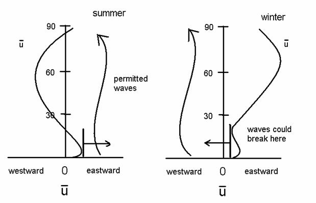
We see that the
permitted waves have cx > ū in the summer, but cx
< ū in the winter. Recall that
for planetary waves. cx < ū, which occurs in the
winter.
Since Lx
>> Lz, k << m.
Thus, we can approximate the equations above as the following:
![]()
since typically, k
<< m (Lx >> Lz). Therefore, we can approximate:
![]()
The level at which
this happens is called the critical level, zc, just as for planetary
waves Note that the wavelength of the
wave goes to 0.
The group velocity
also goes to 0 as cx approaches ū:
![]()
The critical level
is a barrier to the transmission of the wave.
This is the same as for planetary waves.
Recap: We have
described the main wave types that do the forcing – gravity waves and planetary
waves – shown their forcing mechanisms and their allowed propagation. We have shown that gravity waves can
propagate both eastward and westward with respect to the mean flow, whereas
planetary waves can only propagate eastward with respect to the mean flow. The eastward waves give rise to a westerly
acceleration; the westward waves give rise to an easterly acceleration.
Wave breaking.
How then does the
upward propagation of gravity waves and planetary waves create accelerations on
zonal winds in the stratosphere and mesosphere?
In our previous
discussion of gravity waves, we did not take the vertical change in density
into account. When we do this, as we did
for the planetary waves, we get perturbation solutions of the following form:

To see how gravity
waves cause an acceleration, look at isentropic surfaces:
zs 60 km summer; 80 km winter x z
![]()
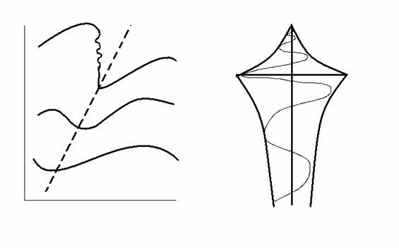
Note that following:
- The phase is downward and eastward in this case.
- Recall that |u’| ~ exp(z/2H) ~ |c - ū|, and that ½ ro u’2 ~ constant. So, the wave amplitude grows
- The isentropic surfaces get progressively more distorted until
the isentropic surface becomes quasi-vertical - ¶q/¶z = 0 – get
convective instability - and the wave breaks.
- Overturning generates local turbulence.
- Most important, the wave can no longer increase in amplitude and
perturbations must decrease, not increase, above this altitude.
- The level at which ¶q/¶z = 0 is called the saturation level, zs.
- When the zonal phase speed, cx approaches the zonal
wind speed, ū, this is the critical level, zc, which is
above zs.
Thus,

Thus, the wave drag
and the gravity wave contribution to the forcing G occurs between the
saturation level and the critical level.
Planetary Wave Forcing
Recall that, for planetary waves, the zonal mean momentum equation and the thermodynamic energy equations have the form:
![]()
![]()
where F is the Eliassen-Palm
(EP) flux, which arises from large-scale eddies, and X is the forcing from the
small-scale eddies, like gravity wave drag.
G is the total zonal drag force. F
= jFy + kFz , where the two components are
given by:
![]()
If there are no
diabatic effects, if the waves are steady and linear and the flow is
conservative, then ¶ū/¶t = ¶T/¶t = 0, which
implies that the mean meridional velocities are also equal to 0. Thus, there is no meridional circulation.
This concept is
called the non-acceleration theorem.
Remember that we
defined a perturbed quasi-geostrophic potential vorticity as:

where the subscript
“g” means geostrophic.
After some work, we
arrive at the expression:
![]()
so that:
![]()
Examine the terms
in this equation.
1.
time-rate-of-change of the zonal mean wind
2.
residual Coreolis force
3.
the northward eddy flux of the potential vorticity
4.
small scale forcing
5.
total forcing
Note that is the
northward eddy flux of potential vorticity is non-zero only if the planetary
wave is either growing or shrinking in time.

We multiply by
![]()
and take the zonal
average to get the equation:

Where the first
term is the time-rate-of-change of the wave activity density:

If the waves are
steady, then ¶A/¶t = 0.
If the waves
areadiabatic and inviscid, then D = 0.
Thus the divergence of the Eliassen-Palm Flux is zero.
So, we come to some
conclusions regarding planetary wave forcing:
- Planetary waves forcing exists only when Ñ·F ≠ 0.
- F is usually directed upward and toward the
equator.
- F is parallel to the group velocity of
coherent waves.
___
for ¶A/¶t > 0, Ñ·F = ro (v’q’) < 0.
Thus, if q’ > 0,
then v” < 0. Thus growing waves
transport potential vorticity equatorward.
In this sense, the growing planetary waves tend to smooth out the mean
potential vorticity distribution.
The Quasi-Biennial Oscillation (QBO)
The QBO is an equatorial oscillation of the
zonal winds, as seen in the figure from the University of Reading
(www.ugamp.rdg.ac.uk/hot/ajh/qbo.htm).
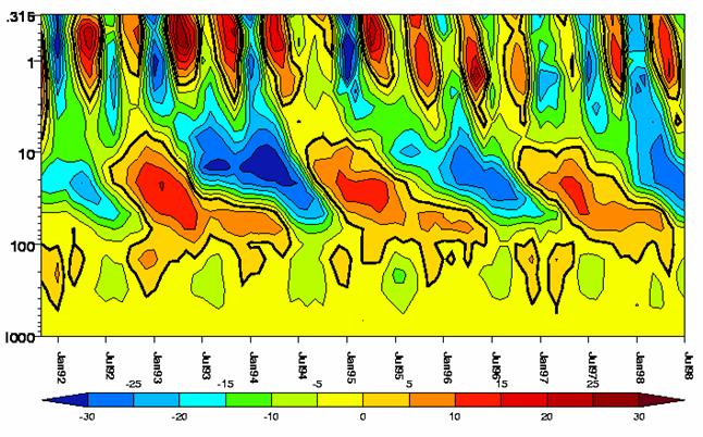
Its main characteristics
are the following:
· The easterlies and westerlies propagate down with time.
· This downward motion progresses at about 1km/month.
· The wind strength decreases as the easterlies or westerlies move to lower altitudes.
· The oscillation’s period is 20 to 36 months, with a mean of ~ 28 months, but with considerable variability in period and amplitude.
· The easterlies and westerlies begin near 10mb and descend to 100mb.
· The maximum amplitude of 40 to 50m/s is seen at 20mb.
· Easterlies are generally stronger than westerlies.
· Westerly winds dwell longer than easterly winds at higher levels while at lower levels, the easterlies dwell longer.
· The westerlies descend faster than the easterlies.
· The transition between westerly and easterly regimes is often delayed between 30 and 50mb.
· The QBO is most prominent below 10 mb, while the Semi-Annual Oscillation is most prominent above 10 mb, as seen in the figure.
The latitudinal extent of the QBO is seen in the second figure from the University of Reading. The figure is the oscillations at 10 mb.
Why do we care about the QBO?
· The QBO seems to influence hurricane activity and is used in hurricane activity prediction. Hurricane activity is greater for the westerly (eastward) phase at lower altitudes than the easterly (westward) phase.
· Tropical cyclones in the northwest Pacific are more frequent during the westerly phase of the QBO.
· The QBO is coupled to ENSO; ENSO predictions use predictions of the QBO winds at 30 mb and 50 mb.
· The QBO influences the strength of the polar ozone loss, with worse ozone loss occurring in the westerly phase at lower altitudes.
· The decay and spread of volcanic injections into the stratosphere depends on the phase of the QBO.
The forcing mechanism for the QBO.
Before we can diagram the forcing mechanism for the QBO, we must talk a little bit about equatorial waves. I will not talk about the wave equations and dispersion relations, like I did before. But rather, I will simply describe the waves that are involved.
Equatorial waves propagate vertically and zonally, but they are trapped to within ±15o latitude of the equator.
Two types of waves are important:
· Rossby-gravity waves – have meridional motion and westward phase speed with respect to the mean flow.
· Kelvin waves – internal gravity waves, with no meridional motion, but with phases that propagate eastward with respect to the mean zonal wind and downward.
Both types of waves are generated by large-scale cumulus convection.
Let’s examine the properties in more detail.
|
property |
Kelvin wave |
Rossby-gravity wave |
|
period (2p/w) |
15 days |
4-5 days |
|
zonal wavenumber (s=ka cosj) |
1-2 |
4 |
|
vertical wavelength (2p/m) |
6-10 km |
4-8 km |
|
phase speed |
+25 m s-1 |
-23 m s-1 |
|
observed when ū is: |
easterly (west) max.:–25 ms-1 |
westerly (east) max: +7 m s-1 |
|
observed amplitudes u’,v’,T’ |
8 m s-1, 0, 2-3 K |
2-3 m s-1, 2-3 m s-1, 1 K |
|
inferred amplitudes (F’/g, w’) |
30 m, 1.5x10⁻³ m s-1 |
4 m, 1.5x10⁻³ m s-1 |
|
~meridional scales |
1300-1700 km |
1000-1500 km |
The forcing of the QBO was explained by Alan Plumb in 1984.
Wave propagate upward until they hit a critical line (cx= ū), where they are damped, depositing momentum. The Kelvin waves deposit eastward (westerly) momentum; the Rossby-gravity waves deposit westward (easterly) momentum. Starting with Figure 4(a), from the University of Reading webpage, both the Rossby-gravity waves (blue) and the Kelvin waves (red) are being damped at low altitudes.
(a) Where the Kelvin waves deposit eastward momentum just below and at the critical line, the mean zonal wind increases and moves down. The same is happening for the Rossby-gravity waves, but at a higher altitude.
(b) Eventually, the eastward zonal wind moves low enough that it dissipates, and the Kelvin wave can propagate all the way to 10 mb, where it can be absorbed.
(c) Now the Rossby-gravity waves are absorbed at very low altitudes and the westerly (eastward) phase is descending because of absorption of Kelvin waves.
(d) Rossby-gravity waves are absorbed at very low altitudes, while Kelvin waves are absorbed higher up.
(e) Rossby-gravity waves are now propagate high into the stratosphere while Kelvin waves are absorbed increasingly lower in altitude.
(f) Both are now absorbed, with the Kelvin waves being absorbed lower in the stratosphere. And we start all over again.

Fig 4. Plumb's analog of the QBO in six stages. Wavy blue and red lines indicate penetration of easterly and westerly waves.
In Fig. 4(a) both easterly and westerly maxima are descending as the upward propagating waves deposit momentum just below the maxima. When the westerly shear zone is sufficiently narrow, viscous diffusion destroys the westerlies and the westerly waves can propagate to high levels through the easterly mean flow, Fig. 4(b).The more freely propagating westerlies are dissipated at higher altitudes and produce a westerly acceleration leading to a new westerly regime, Fig. 4(c). Fig. 4(d) shows both regimes descending downwards until the easterly shear zone becomes vulnerable to penetration and the easterlies can then propagate to high altitudes, Fig. 4(e), and so onto the formation of a new easterly regime in Fig. 4(f).
Equatorial
Semi-Annual Oscillation (SAO).
The sun passes over the equator twice a year, giving rise to a semiannual signal. However, thermal forcing from the sun is inadequate to actually cause the observed wind changes; eddy forcing must be the cause.
· The SAO occurs at altitudes above the QBO.
· It has two separate oscillations: one in the stratosphere and one in the mesosphere, with an amplitude minimum near 65 km.
· The amplitudes in the stratosphere and mesosphere are comparable, but are 6 months out of phase.
· Oscillations are limited to ±25o of the equator.
· Oscillations appear first in the mesosphere and then propagate downward.
· stratospheric oscillation: easterly maximum at solstices, westerly maximum at equinoxes.
· mesospheric oscillation: westerly maximum at solstices, easterly maximum at equinoxes.
· While
the westerlies are likely to be driven by Kelvin waves, it is not clear what
drives the easterlies.
Tracer
Transport.
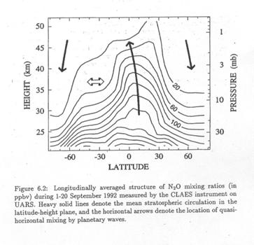
We now have a pretty good sense of how air moves through the stratosphere, as the figure from Plumb shows:
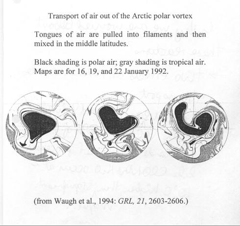
A tracer labels an air parcel. To be a good tracer, it must have a gradient in either time or space. For space, the gradient is typically equator to pole and with altitude. For time, the gradient is either a seasonal cycle or a trend. In either case, the gradient must be established and exist on a timescale that is long compared to the transport phenomenon of interest. Thus, a tracer of the polar vortex must exist on a time scale that is longer than the planetary wave motions (~1-2 weeks) that distort the polar vortex and cause it to shed air into the midlatitudes. This condition requires tracers that are sufficiently long-lived that they do not change their values as they are transported. On the other hand, if the tracer is very long lived, then the gradient will never be established. Without a gradient, we cannot determine transport. Thus, we want a “quasi-conservative” tracer.
We have two types: dynamical tracers and chemical tracers.
Dynamical tracers:
· Potential vorticity
· Potential temperature
These two quantities change over the course of weeks. PV changes by either diabatic heating and cooling or wave-breaking. Potential temperature changes by diabatic heating and cooling.
Chemical tracers with spatial gradients:
· Ozone: Good only in the lower stratosphere or at high latitudes where its chemical lifetime is much longer than its dynamical lifetime.
· N2O – destroyed by photolysis; has a 120 year lifetime.
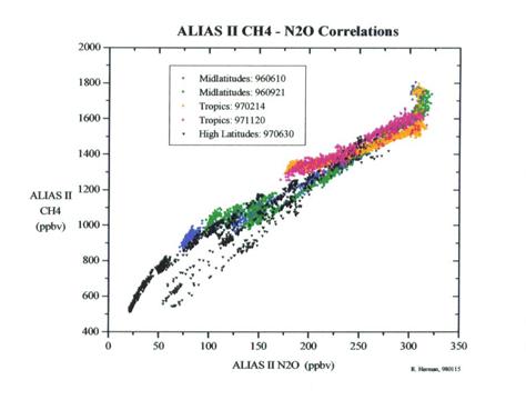
· CH4 - destroyed by reaction with OH; has a 15 year lifetime. Because CH4 and N2O are destroyed by processes that are related, the mixing ratios of the two chemicals (and actually many more) have a fairly compact relationship relative to each other.
· CFCs – destroyed by photolysis; have lifetimes of ten’s to hundreds of years.
Chemical tracers with temporal gradients:
· CO2 – seasonal cycle and trend
· SF6 – trend of 7% increase per year
· H2O – seasonal cycle
Both CO2 and H2O are good for looking at the ascent of air in the tropical lower stratosphere, which is quasi-isolated from the midlatitude lower stratosphere by dynamical barriers.
Trends are very good for determining the mean age of an air parcel in the stratosphere. To determine the mean age, we need only look at the mixing ratio of a chemical that is lost only slowly in the stratosphere – such as CO2 or SF6 – and look back in time to when that chemical had that mixing ratio in the tropical upper troposphere. Typical mean ages for the stratosphere are 3 to 7 years for air parcels at high latitudes. The higher the air parcel has risen, the greater will be its mean age.
For transport out of (or into) the polar vortex, it turns out that N2O and Potential Vorticity give us almost exactly the same information. We can see from the figure that air is transported out of the polar vortex by planetary waves that get increasing non-linear so that pieces are literally sheered off.
Stratosphere
– Troposphere Exchange.
We can look at the exchange of gases between the stratosphere and the troposphere on many spatial scales from global to local (~100 km). We will examine the processes that lead to stratosphere-troposphere exchange over all of these scales.
Large scale.
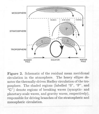
The current thinking on the general transport through the stratosphere is that it is driven by breaking waves slowing down the mean zonal flow, resulting in a poleward drift of the air parcels, which thus must descend by mass continuity. This descent must be, for the most part, back into the troposphere.
A picture from Holton’s review shows the basic processes that are involved.
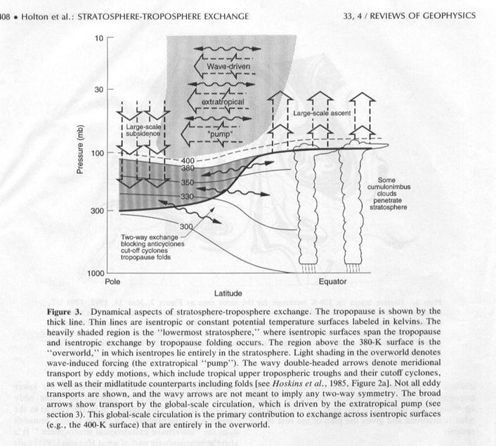
We can see the general stratospheric circulation, with air rising in the tropical region, being transported by the extratropical pump toward high latitudes, where it must again sink. This path is the one that I have been trying to stress in class.
We also see a shorter path between the tropical upper troposphere and the higher latitudes: isentropic flow into the lowermost stratosphere. Because these air parcels never rise very high into the stratosphere, it is difficult to imagine that they have much of a role in stratospheric chemistry. Indeed, models show that the lifetimes of these air parcels in the stratosphere are measured in months, not years. Thus, when we think about transport into and out of the stratosphere, a better surface to consider is the lowest potential temperature surface that is entirely in the stratosphere, about 380-400 K potential temperature.
So, how much circulation do the eddies cause? What is the mass flow through the stratosphere?
|
Mass flux across the 100-hPa surface in 108 kg s-1 |
|||
|
|
DJF |
JJA |
Annual Mean |
|
NH extratropics |
-81 |
-26 |
-53 |
|
Tropics |
114 |
56 |
85 |
|
SH extratropics |
-33 |
-30 |
-32 |
Note that the NH downward mass flux is much greater than the SH downward mass flux. Why is this?
Small scale processes near the tropopause: The midlatitudes and subtropics.
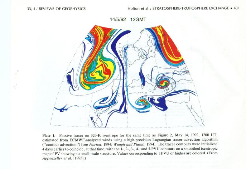
The primary mechanism is tropospheric folding. Tropospheric folds are tongues of stratospheric air that get drawn into the troposphere around jet streams. The generally occur in winter and spring. They are observed near upper-tropospheric jets, usually downstream of a ridge. As the fold reaches downward into the troposphere, it can become irreversibly stretched to smaller and smaller scales, eventually becoming irreversibly mixed with the tropospheric air. Of course, such air brings with it higher values of ozone. This stratospheric ozone is thought to contribute about 10% of the global tropospheric ozone.
A second mechanism is cut-off cyclones. In this case, the tropopause is anomalously low and air is mixed by shearing processes.
Small scale processes near the tropopause: The tropics
This has been a subject of much debate for a few decades, and it is still ongoing. Possible mechanisms include:
· Overshooting
convection in
· A stratospheric fountain. The air is lifted into the stratosphere by heating.
· Observations show that the air enters the stratosphere pretty much year-round. This can be seen by the seasonal cycle of CO2 and H2O.
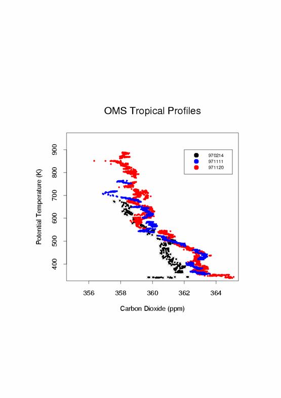
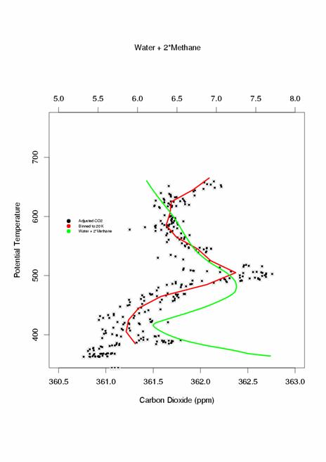
We can see from these CO2 data that the air is entering the stratosphere pretty much all year round, although the cycle is compressed somewhat at some times relative to others, indicating that the air does not flow uniformly into the stratosphere.