Meteo 532 Atmospheric Chemistry

Fall 2003

Problem set 2 Solutions

Problem 2.1. Energy and potentialtemperature. Assume that we have a 1-kg air parcel at 70^oN latitude. Use Figure 2.3 to do this problem. Why should you use the specific heat, constant pressure, to do this problem?

a. How much energy is required to raise it from 0 to 5 km?

b. How much energy is required to raise it from 10 to 15 km?

c. What does this tell you about the relative stability of the troposphere and the stratosphere?

Solution. We use c_p because the air parcel’s volume is not contained and can expand. Futhermore, we are using potential temperature, which is the temperature that an air parcel would have at 1000 hPa. The change in temperature is therefore just the change in potential temperature, and the energy required for the 1-kg parcel to go through from one potential temperature surface to another requires only that we know Dq and c_p in the equation: E_i_-j = 1 kg (c_p) Dq.

a. 0-5 km. Dq = 25 K, which mean E_0-5 = 1 kg x 1040 J K^-1 kg^-1 x 25 K = 26 kJ

b. 10-15 km. Dq = 80 K, so that E_10-15 = 1 kg x 1040 J K^-1 kg^-1 x 80 K = 83 kJ

c. Because it requires more than 3 times the energy to raise a 1-kg air parcel 5 km in the stratosphere compared to the troposphere, and because the local source of heating at 10 km is so much smaller than the local source of heat at 0 km, the stratosphere must be much more stable than the troposphere.

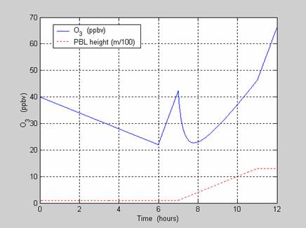
Problem 2.2. A simplified morning rush hour problem. O₃’s mixing ratio at the surface is influenced not only by the chemical production and loss of ozone, but also by the height of the planetary boundary layer. The net production of ozone can be approximated by the following function: from midnight (0) to 6 in the morning, the production rate of ozone, dO₃/dt = -3 ppb/hr; (It’s lost by deposition to the surface), from 6 to 12, dO₃/dt = 20 ppb/hr (It’s created by chemistry). At midnight, 0, χ_O3 = 40 ppbv. The planetary boundary layer height, h, can be approximated by the function: from 0 to 7, h = 100 m; from 7 to 11, dh/dt = 300 m/hr; from 11 to 12, dh/dt = 0.

a. Using a computer program or Excel, plot O₃’s surface mixing ratio in ppb. Assume that there is no horizontal advection (i.e., no wind).

MATLAB m-file program called o3calc.m

% o3calc.m finds and plots the time-dependent O3 change due to chemical

% production and boundary layer growth.

h0 = 100;

o30 = 40;

dt = 0.5/60;

% I choose 0.5-minute intervals for the time step.

% At each 0.5-minute step, we add the chemically produced ozone to the existing ozone

% and then dilute the ozone by the ratio of the growth of the PBL height from

% the begining to the end of the 5-minute interval.

% We are assuming that ozone is being produced throughout

% the PBL as it grows.

o3(1) = o30 - 3*dt;

% For midnight to 6 am

for i= 2:719

t(i) = i/120;

h(i) = h0;

o3(i) = (o3(i-1) - 3*dt)*(h0./h(i));

end

% For 6 to 7 am

for i= 720:839

t(i) = i/120;

h(i) = h0;

o3(i) = (o3(i-1) + 20*dt)*(h(i-1)./h(i));

end

% For 7 to 11 am

for i= 840:1320

t(i) = i/120;

h(i) = h0 + 300*(t(i)-7);

o3(i) = (o3(i-1) + 20*dt)*(h(i-1)./h(i));

end

% For 11 am to noon

for i= 1321:1440

t(i) = i/120;

h(i) = h(1320);

o3(i) = (o3(i-1) + 20*dt)*(h(i-1)./h(i));

end

plot(t,o3,t,h/100,'r:')

xlabel('Time (hours)')

ylabel('O_3 (ppbv)')

legend('O_3 (ppbv)','PBL height (m/100)')

grid

Problem 2.3. Dispersion in a Gaussian plume. Using thePasquill turbulence types and the Briggs formulae, estimate the Gaussian plume expansion for the conditions at 10 am, 3 pm, and 10 pm on Thursday, 18 September. Determine the Gaussian equation and get the expansion at 1 km. You can get the wind speed at: http://www.srh.noaa.gov/data/forecasts/PAZ019.php?warnzone=paz019&warncounty=pac027. Explain why you chose the Pasquill turbulence types that you did for the three different times.


time	wind speed (m/s)	conditions	Pasquill type	s_y (m) @ 1 km	s_z (m) @ 1 km
10 am	3.6	mostly overcast; slight insolation	C	105	73
3 pm	6.3	overcast; slight insolation	D	76	38
10 pm	9.4	overcast	D	76	38

I use the Briggs equations to calculate the dispersion in the y and z directions. I assume rural conditions.

	s_y (m)	s_z (m)
C	0.11 x (1 + 0.0001 x)^-1/2	0.08 x (1 + 0.0002 x)^-1/2
D	0.08 x (1 + 0.0001 x)^-1/2	0.06 x (1 + 0.0015 x)^-1/2

At 10 am, the smoke stack plume spreads fairly quickly, while it is much smaller at 3 pm and 10 pm.

10 am:

3 pm and 10 pm: