Meteorology 532 – Atmospheric Chemistry

Problem Set # 3 - Solutions

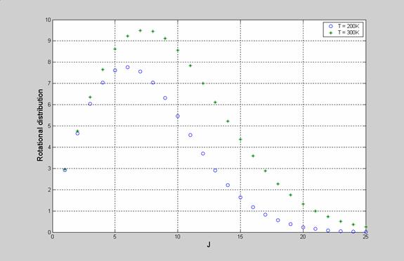
Problem 3.1. Rotational distribution of NO. Use the equation given above to determine the ratio of NO molecules in the different J levels (J = 0, 1, 2, 3, …) compared to the J=0 level for temperatures of 200 K and 300 K. Plot the ratios in each J level as a function of J for the two temperatures. B = 1.7 cm^-1 for ground-state NO.

We can find the distribution function with the expression:

where h = 6.626x10^-34 J s; c = 3x10⁸ m s^-1; k = 1.38x10^-23 J K^-1; and B = 170 m^-1.

We use the following program to do the calculations up to J = 25.

% rotboltz.m calculates the rotational Boltzmann distribution, relative to

% J = 0, for the temperatures 200 K and 300 K

h = 6.626e-34;

c = 3.0e8;

k = 1.38e-23;

B = 170;

factor = B*h*c/k;

for i = 1:25

J(i) = i;

end

f200 = (2*J+1).*exp(-(factor.*J.*(J+1)./200));

f300 = (2*J+1).*exp(-(factor.*J.*(J+1)./300));

% plot the two distributions

plot(J,f200,'o',J,f300,'*','markersize',6)

grid

xlabel('J','fontsize',14)

ylabel('Rotational distribution','fontsize',14)

legend('T = 200K','T = 300K')

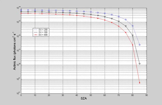
Problem 3.2. Dependence of actinic flux on overhead ozone. Ozone’s absorption cross section at 310 nm is 1x10^-19 cm^-2. The actinic flux from 309.5 to 310.5 nm is 1.2x10¹⁴ photons cm^-2 s^-1. Plot the actinic flux at Earth’s surface as a function of solar zenith angle for overhead ozone of 200 DU, 300 DU, and 400 DU. You can assume that the ozone column consists of a constant concentration spread uniformly between 15 and 35 km. Use the corrected expression for I(z) given above. Calculate the column density and then determine the concentration from 15 to 35 km that sums to the column density you determined.

The actinic flux within 1 nm of 310 nm is 1.2x10¹⁴ photons cm^-2 s^-1. 100 DU is equivalent to 1 mm of pure ozone at STP, or 2.69x10¹⁹ molecules mm^-1 cm^-2, or 2.69x10¹⁸ molecules cm^-3. Since we are distributing this total concentration not in 1 cm of height, but of Dz = (35-15)(1000)(100)(10) = 2x10⁶ cm of height, the concentration in any cubic cm is 1.34x10¹² molecules cm^-3 for 100 DU. We are doing the calculations in cm units.

The equation we use is I(z) = I_infinity exp(∫(- sec(SZA) s_z n(z) (z) dz).

Because we have such a simplified atmosphere, we can rewrite this expression as:

I(0) = I_infinity exp(-s n(z) Dz sec(SZA))

The resulting computer program is:

% fo3sza.m determines the actinic flux for different ozone

% columns

%

dz = 2e6; n100 = 1.34e12; sigma = 1e-19; Finf = 1.2e14;

%

factor = sigma*dz*n100;

%

for i = 1:18

sza(i)=5*(i-1);

end

%

szarad = sza/57.296;

%

F200 = Finf*exp(-factor.*(200/100)./cos(szarad));

%

F300 = Finf*exp(-factor.*(300/100)./cos(szarad));

%

F400 = Finf*exp(-factor.*(400/100)./cos(szarad));

%

semilogy(sza,F200,'b:',sza,F300,'k',sza,F400,'r.-',...

sza,F200,'bo',sza,F300,'kv',sza,F400,'r*','markersize',6)

grid

xlabel('SZA','fontsize',14)

ylabel('Actinic flux (photons cm^{-2} s^{-1}','fontsize',14)

legend('DU = 200','DU = 300','DU = 400')

Problem 3.3. Estimate the photolysis frequency for the reaction

O₃ + hn ® O(¹D) + O₂ at 40 km and 0 km altitude. Use Figure 3.4 to determine the actinic flux and JPL to get the O₃ cross sections and the O(¹D) quantum yields. I suggest using a computer program or spread sheet to do a sum over wavelength.

My sum over wavelength consists of values taken every 10 nm from 185 nm to 365 nm. I found the actinic fluxes at 0 km and 40 km by taking estimated values from the graph. I estimated the cross sections for every 10 nm.

The results are: JO₃ = 3.5x10^-5 s^-1 at 0 km and 1.6x10^-3 at 40 km. These values are quite close to the values obtained with the actual numbers and not just estimates like I used.

The computer program that I used is:

% jo3.m caculates the photolysis frequency for ozone photolysis into

% O(1D).

%

% Do the calculation for every 10 nm. Assume both temperatures are 273 K

%

for i = 1:19

wl(i)=175 + 10*i;

end

%

cs = [58 35 35 100 300 650 1040 1140 960 550 200 80 18 5 1.2 0.3 0.06 0.01 0.005];

sigma = cs*1e-20;

F_40 = [1e9 3e11 9e11 3e12 2e12 8e11 3e11 2e11 1.5e12 4e12 2e13 7e13 1e14 1.5e14 ...

2e14 3e14 3e14 4e14 5e14];

F_00 = [0 0 0 0 0 0 0 0 0 0 0 6e10 1.5e13 8e13 1.5e14 2e14 2e14 2.5e14 3e14];

%

% QE values from JPL 14, except transitions at 315 and 325, which came from

% a graph in Finlayson-Pitts and Pitts

QE = [.9 .9 .9 .9 .9 .9 .9 .9 .9 .9 .9 .9 .9 .2 .1 .08 0 0 0];

%

J_0 = sum(F_00.*sigma.*QE*10)

J_40 = sum(F_40.*sigma.*QE*10)

%

% I use the figures to check to make sure that I haven’t made any mistakes in my estimates.

%

figure

semilogy(wl,F_40,wl,F_00)

xlabel('wavelength (nm)')

ylabel('actinic flux (photons cm^{-2} s^{-1} nm^{-1}')

%

figure

semilogy(wl,sigma)

xlabel('wavelength (nm)')

ylabel('cross section (cm^2)')

%

Problem 3.4. Exothermic or endothermic? Determine if the following reactions are exothermic or endothermic and by how much:

1. O(³P) + H₂O ® OH + OH

DH = 2(37.2) – (-241.8 +249.2) = 67 kJ mole^-1 endothermic

2. O(¹D) + H₂O ® OH + OH

DH = 2(37.2) – (-241.8 + 438.0) = -121.8 kJ mole^-1 exothermic

3. NO + NO + O₂ ® NO₂ + NO₂

DH = 2(34.2) – 2(91.3) = -114.2 kJ mole^-1 exothermic

4. HO₂ + O₃ ® OH + 2O₂

DH = (37.2+0)-(13.8+141.8) = -118.4 kJ mole^-1 exothermic

5. OH + CF₄ ® HOF + CF₃

DH = (-98.3-465.7)-(37.2-933.2) = 332.0 kJ mole^-1 endothermic

6. Cl + CH₄ ® HCl + CH₃

DH = (-92.3+146.6)-(121.3-74.5) = 7.5 kJ mole^-1 endothermic

When entropy is considered, this reaction occurs spontaneously.

7. Br + CH₄ ® HBr + CH₃

DH = (-36.3+146.6)-(111.9-74.5) = 72.9 kJ mole^-1 endothermic

Problem 3.5. The actual number of molecules that hit the surface of atmospheric aerosols is equal to the flux, F, times the aerosol surface area per volume of air, A, where A has units of cm² cm^-3 of air. If we assume the all the molecules stick, then the molecule loss rate is given by dn/dt = - FA = -1/4 <v>A n.

What is the loss rate of HCl in the Antarctic ozone hole for the following conditions: p = 50 hPa; T = 195 K; c_HCl = 1 ppbv; and the surface area density, A, = 10^-8 cm² cm^-3? Assume that all HCl sticks. You need to get [HCl] in molecules cm^-3, which is the same thing as n in the equation above.

d[HCl]/dt = - ¼ <v>A [HCl]

<v> = 145.5 x (T in K/M in g mole^-1)^1/2 m/s = 14550*(195/36.5)^1/2 = 3.36x10⁴ cm/s

[HCl] = 2.69x10¹⁹(50/1013)(273/195) (1x10^-9) = 1.85x10⁹ molecules cm^-3.

d[HCl]/dt = -1/4 x 3.36x10⁴ x 10^-8 x 1.85x10⁹ = 1.6x10⁵ molecules cm^-3 s^-1

Problem 3.6. For a temperature of 250 K and pressure of 200 hPa, determine the following bimolecular rate coefficients:

1. OH + CH₄ ® H₂O + CH₃

k = 2.45x10^-12 exp(-1775/250) = 2.02x10^-15 cm^-3 molecule^-1 s^-1

2. OH + CO ® H + CO₂

k = 1.5x10^-13(1+0.6(200/1013)) = 1.7x10^-13 cm^-3 molecule^-1 s^-1

3. O(¹D) + H₂O ® 2OH

k = 2.2x10^-10 cm^-3 molecule^-1 s^-1

4. NO₂ + O₃ ® NO₃ + O₂

k = 1.2x10^-13 exp(-2450/250) = 6.6x10^-18 cm^-3 molecule^-1 s^-1

Problem 3.7. Termolecular reaction rate coefficients. On a log-log plot, plot the effective bimolecular rate coefficients (cm^-3 molecule^-1 s^-1) for the following reactions:

1. OH + NO₂ + M ® HNO₃ + M
2. NO₂ + NO₃ ® N₂O₅ + M
3. H + O₂ + M ® HO₂ + M
4. ClO + NO₂ + M ® ClONO₂ + M

Calculate these values for M = 3x10¹⁷ to 3x10¹⁹ molecules cm^-3. I suggest using a spreadsheet or computer program.

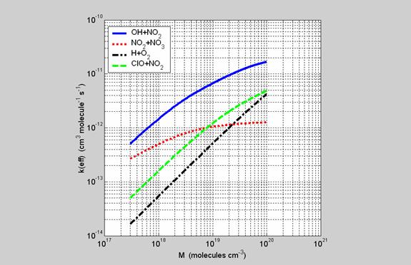
Note that only NO₂+NO₃ ® N₂O₅ is approaching its high pressure limit and that only H+O₂ ® HO₂ is pretty much in its low pressure limit for the entire range of the atmosphere. We can see this quickly on the log-log plot because its slope remains very close to 1 over the entire range.

The following program was used to calculate these rate coefficients:

%termocalc.m calculates the termolecular rate coefficients at 300 K for

% 3x1017 to 3x1019 molecules cm-3

%

% OH + NO2 + M --> HNO3 + M

ko1 = 2.0e-30;

ki1 = 2.5e-11;

% NO2 + NO3 + M --> N2O5 + M

ko2 = 2.0e-30;

ki2 = 1.4e-12;

% H + O2 + M --> HO2 + M

ko3 = 5.7e-32;

ki3 = 7.5e-11;

% ClO + NO2 + M --> ClONO2 + M

ko4 = 1.8e-31;

ki4 = 1.5e-11;

%

%

for i = 1:998

M(i) = (2 + i)*1e17;

end

%

rk1 = (ko1*M)/ki1;

k1 = ((ko1.*M)./(1+rk1)).*0.6.^(1./(1+(log10(rk1)).^2));

%

rk2 = (ko2*M)/ki2;

k2 = ((ko2.*M)./(1+rk2)).*0.6.^(1./(1+(log10(rk2)).^2));

%

rk3 = (ko3*M)/ki3;

k3 = ((ko3.*M)./(1+rk3)).*0.6.^(1./(1+(log10(rk3)).^2));

%

rk4 = (ko4*M)/ki4;

k4 = ((ko4.*M)./(1+rk4)).*0.6.^(1./(1+(log10(rk4)).^2));

%

loglog(M,k1,'b',M,k2,'r',M,k3,'k',M,k4,'g')

xlabel('M (molecules cm^{-3})')

ylabel('k(eff) (cm^{3} molecule^{-1} s^{-1})')

grid

legend('OH+NO_2','NO_2+NO_3','H+O_2','ClO+NO_2')

axis([1e17 1e21 1e-14 1e-10])

axis('square')