2

2. The Atmosphere

2.1. General Composition

The main constituents, their molecular weights, and volume mixing ratios are in Table 2.1.

Table 2.1 Major constituents in Earth’s present atmosphere
constituent	molecular mass (g/mol)	mixing rato (mol mol^-1)	Role in atmospheric chemistry?
nitrogen (N₂)	28.013	0.7808	as collision partner only
oxygen (O₂)	31.998	0.2095	major roles
argon (Ar)	39.948	0.0093	no role
carbon dioxide (CO₂)	44.010	0.000356	minor role
neon (Ne)	20.183	0.0000182	no role
water vapor (H₂O)	18.015	2x10^-6 to 0.05	major roles

One role for these major constituents is to act as collision partners with other molecules. We will see that these collisions are important some types of chemical reactions that occur in the atmosphere. Nitrogen and oxygen have the largest roles because they are most abundant, but water vapor can have a surprisingly large influence itself.

With the exception of oxygen and water vapor, the primary constituents involved in atmospheric chemistry exist in the atmosphere in ppmv or less. These constituents are often called trace species because their abundance is so much smaller than that of nitrogen or oxygen.

2.2. Important meteorological concepts

Atmospheric chemistry is ultimately driven by sunlight. However, it is also heavily influenced by temperature and pressure. In addition, the transport of constituent emissions from Earth’s surface has a tremendous influence on the evolution of pollution and atmospheric chemistry. It is necessary to understand some basic meteorological concepts before tackling atmospheric chemistry itself.

2.2.1 Overall structure – troposphere, stratosphere

2.2.1.1. Temperature

The atmosphere’s vertical temperature structure dictates the vertical transport of constituents (Figure2.1).

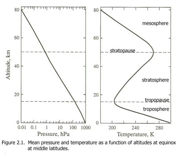
The temperature decreases throughout the troposphere to a local minimum at the tropopause of about 200 K. The technical definition of the tropopause is the lowest altitude above which the temperature does not increase by more than 2 K for 2 km. Above that altitude, the absorption of solar energy by stratospheric ozone heats the air, causing the temperature to rise. The ozone concentration decreases dramatically above 40 km, so that solar heating of the air above 50 km is less and the temperature again decreases.

While this general temperature pattern holds throughout the atmosphere, the exact structure changes with latitude and season (Figure 2.2).

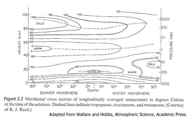
Notice that

· the tropopause is higher in the tropics than at higher latitudes

· the wintertime lower stratosphere is quite cold

· the tropical tropopause region is colder than anywhere in the lower stratosphere, except at wintertime high latitudes.

2.2.1.2 Pressure

Atmospheric gases can generally be treated as Ideal Gases, which behave according to the Ideal Gas Law:

(2.1)

where V is the volume, n is the number of moles, and R is the Gas Constant, which equals 8.134 J mol^‑1 K^-1. The density of the gas is thus given by the equation:

(2.2)

where M_air is the molecular mass of air, which equals 0.029 kg mol^-1 and r is in kg m^-3.

From a simple mass balance of forces on a slab of air, the change of pressure with height can be derived as the equation:

(2.3)

Temperature changes by less than a factor of two over the entire atmosphere up to 80 km, while the pressure decreases with height by several orders of magnitude. As a result, to first approximation, we can assume that T is independent of altitude and integrate Equation 2.3 to give the expression:

(2.4)

where p_o is the pressure at Earth’s surface and H = R T/M_airg is the atmospheric pressure scale height, which equal to about 7-8 km. Thus, the pressure decreases by 1/e every 7-8 km.

2.2.1.3 Potential Temperature

Recall that an adiabatic process for a volume of an ideal gas is one in which the energy of the gas in the volume is conserved- energy flow neither in nor out. If an ideal gas is expanded or compressed adiabatically, pressure, temperature, and volume change in ways that maintain certain relationships. The relationship – one of the three Poisson relations - is the equation for the relationship between pressure and temperature:

(2.5)

where g = c_p/c_v, specific heats at constant pressure and volume per unit mass of air. The potential temperature, θ, is defined as the temperature an air parcel would have if it were brought adiabatically to a pressure of 1000 hPa:

(2.6)

Air parcels can rise and fall adiabatically for only so long before diabatic effects such as radiative heating and cooling or phase changes take place. None-the-less, potential temperature is a powerful concept that enables the concept of stability.

The average potential temperature as a function of height and latitude shows little gradient in the troposphere, with a considerable increasing gradient in the stratosphere (Figure 2.3).

2.2.1.4 Stability

The stability of an air parcel with regards to its environment depends on its air density compared to the air density of the environment. If it is less dense, either by being warmer or by having more water vapor, then it will rise. If it is more dense, either by being cooler or by having less water vapor, it will sink.

When a dry air parcel rises adiabatically, it expands and cools according the Poission relations. Because we know how the pressure changes, we can find out how the temperature changes using the equation for potential temperature. The result of this manipulation is the equation:

(2.7)

Γ_d is called the dry adiabatic lapse rate.

If, in the atmosphere, the actual temperature change with height decreases less than - Γ_d, then an air parcel given a nudge upward will still be cooler than its surroundings at the higher altitude and it will sink back down to its original position. If it is given a nudge downward, then it will be warmer than its surroundings at the lower altitude and it will rise back to its original position. This condition is said to be stable.

If on the other hand, the actual temperature change with height decreases more than - Γ_d, then an air parcel given a nudge upward will become warmer than its surroundings at the higher altitude and it will continue to rise until it meets an environment where the temperature change with height is less than - Γ_d. This condition is said to be unstable.

We can relate temperature change with height to potential temperature change with height. If the actual potential temperature profile with height is constant, so that dθ/dz = 0, then the actual temperature profile is that of a dry adiabat. This condition is called neutral.

If for an atmospheric layer dθ/dz > 0, then that layer is stable.

If for an atmospheric layer dθ/dz < 0, then that layer is unstable.

Some examples of conditions that occur in the atmosphere are shown in Figure 2.4.

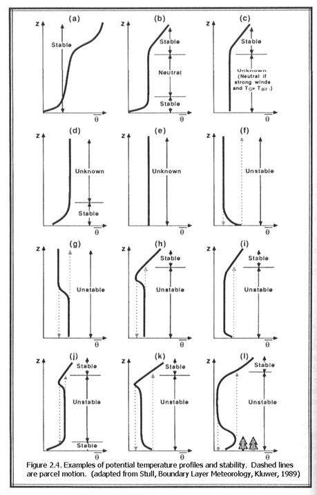
In some cases, it is unknown if the condition is stable or unstable because stability depends on the initial motion and position of the air parcel in question.

If a rising air parcel contains water vapor, its temperature will eventually match its dewpoint temperature and a cloud will begin to form. If air continues to rise in the cloud, the lapse rate becomes smaller because of the latent heat release that comes from the water vapor condensing. The typical moist adiabatic lapse rate is ~6 K km^-1.

Problem 2.1. Energy and potential temperature. Assume that we have a 1-kg air parcel at 70^oN latitude. Use Figure 2.3 to do this problem. Why should you use the specific heat, constant pressure, to do this problem?

            a. How much energy is required to raise it from 0 to 5 km?

            b. How much energy is required to raise it from 10 to 15 km?

            c. What does this tell you about the relative stability of the troposphere and the stratosphere?

2.2.2 Winds

The winds’ speed, direction, and change with height has a huge influence on atmospheric chemistry. We will delve into this subject more as we progress through the course, but for now, I will mention only a few aspects of the wind.

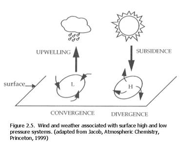
The wind circulates counterclockwise around low pressure and clockwise around high pressure in the Northern Hemisphere. In the Southern Hemisphere, the wind circulates clockwise around low pressure and counterclockwise around high pressure (Figure 2.5). The air converges into a low pressure region and there is upwelling, which can give rise to cloud condensation. The air diverges from a high pressure region as air subsides into a high pressure region, leading to generally clear conditions.

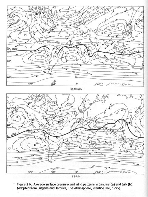
Outside of the tropics, which is between roughly 20^oN and 20^oS, the winds generally move from west to east (Figure 2.6). Thus, intercontinental pollution will tend to travel from Europe to Asia, Asia to North America, and North America to Europe in the Northern Hemisphere. Note that the air flow is much more zonal, and faster, in the winter hemisphere. In the summer the winds tend to slow down and become more meandering, as high pressure regions strengthen. Of particular importance to the Eastern United States in summertime is the presence of the Bermuda high. Clockwise air flow around this high tends to bring air up through the southeastern US into the Northeast. If the air is stagnant, pollution can become severe.

Different parts of the United States are affected by air masses from different directions (Figure 2.6a). Air from western Canada is usually cleaner than air from the Southeast, but there are exceptions, such as large forest fires, which have influenced air quality in the Eastern United States a few times in the last decade.

2.2.3 Planetary Boundary Layer (PBL)

The planetary boundary layer (PBL) is the part of the atmosphere that is in closest contact with Earth’s surface and gaseous emissions from Earth’s surface. Above the PBL is the free troposphere, which is much more decoupled, both chemically and dynamically, from processes that are happening near Earth’s surface. Mixing from near the surface to the PBL’s top and back down again is rapid – typically 30 minutes to an hour. The result is that chemicals that are not too reactive are rapid well mixed throughout the PBL. Their mixing ratios do not vary much with height. During a warm summer’s day, when convection is strong, the PBL height is typically 1-1.5 km over the Eastern United States. Over oceans, the PBL tends to be hundreds of meters high, while over a desert in summertime, the PBL height can be 4 km, as it is in Phoenix, AZ.

The PBL height changes dramatically during a diurnal cycle. In the afternoon, when solar heating and convection are going strong, the PBL is at its maximum height (Figure 2.7). Moisture mixed upward and cooled forms clouds. Mixing of air between the convective mixed layer and free atmosphere occurs in a narrow layer at the top of the PBL, called the entrainment zone. Near sunset, as convection begins to die down, mixing over the convective mixed layer height ceases. As the surface cools by radiation to space, a shallow stable layer forms and becomes decoupled from the air just about it. The stable nocturnal boundary layer is typically 5-10 times smaller than convective mixed layer. The air just above the stable nocturnal boundary layer is sometimes called the residual layer. After sunrise, solar heating again gets convection going. Air from the residual layer is mixed down and air from the stable boundary layer is mixed up, and eventually, they are mixed together.

Why is the PBL height and its diurnal changes so important to atmospheric chemistry? Because air is well mixed throughout the PBL, but is more slowly mixed into the free troposphere, the PBL is the volume of air into which chemicals from the surface are mixed. For a chemical that is emitted at a constant rate all day long into a stagnant airmass, it mixing ratio will be greater when the PBL height is lower, such as at night, than during midday, when the PBL height is at its greatest. Because we are often interested in the mixing ratios of pollutants at Earth’s surface, in the air that we breathe, the PBL height partly controls the mixing ratios of those pollutants.

Understanding the influence of the PBL heights on pollutants is complicated by two main factors. First, as we will see, the chemistry that converts surface pollutant emissions into the pollutants ozone and PM2.5 (particulate matter smaller than 2.5mm in diameter) is non-linear in the concentrations of the surface pollutants. Thus, as the PBL height changes during the day, the efficiency with which the chemistry creates ozone and PM2.5 changes. Second, emissions of many pollutants change during the day. The most striking example is the large pulses of nitrogen oxides, volatile organic compounds (VOCs), and others pollutants that are associated with internal combustion engines and rush hour traffic. Morning rush hour occurs right at the time when the PBL height is changing rapidly, so that changing emissions and non-linear chemistry are interacting.

2.2.5 Dispersion and turbulence

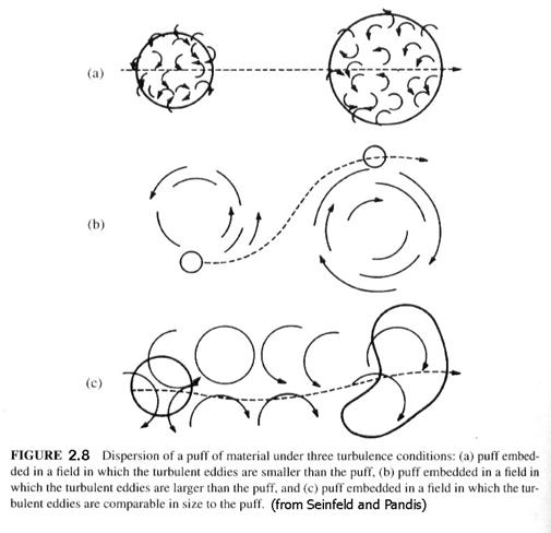
Turbulent motions, or eddies, are responsible for essentially all mixing of atmospheric gases in the atmosphere. Molecular diffusion is dominant in only two domains: the atmosphere above ~110 km, and within a millimeter, or less, of surfaces. Therefore, turbulence has considerable control over the transport and dispersion of atmospheric constituents. We will not delve into turbulence theory here; that’s a different course. But we will use concepts coming out of turbulence to discuss atmospheric dispersion.

Consider emissions of gases or aerosols into the atmosphere. Some emissions occur over a short duration or in puffs. Figure 2.8 shows how turbulence interacts with puffs. First, it can enlarge them with internal turbulence. Second, larger scale turbulence can actually move puffs around. Third, turbulence of a similar scale to the puff can distort it, enlarge it, and move it around. Puffs increase in size with time, as they are mixed with surrounding air. We will not discuss the equations governing the growth of puffs. Instead, we will concentrate on steady emissions, such as those from a power plant or even a large urban area.

Consider a plume (Figure 2.9). After it is emitted, it will flow downwind. This wind direction changes at the source and as the plume moves downwind. At the same time, the plume can be mixing with the surrounding air by turbulence, thus expanding. The instantaneous boundary meanders. Over 10 minutes, the wind has moved the plume over a wider range of angles. The 10-min average boundary, which contains all the volume in which the plume has been, is now larger. The 1-h average boundary is even greater. If the emissions are at a constant rate, then in the averaging process, the peak concentration on the centerline comes down, but it spreads out in a way that preserves the total amount.

Upon averaging, the distribution of concentrations of the plume’s constituents approaches that of the Gaussian, or normal, distribution:

(2.8)

where n is the concentration, n is the mean value, and s is the standard deviation. The (2π)^-1 is a normalization factor that makes the integral of p equal to 1. We can determine the fraction of the plume’s constituent that is between -s and +s by integrating the probability distribution. We find that the fraction of the plume constituent is 68% between these limits. For ±2s, the fraction contained is 95%. The standard deviations of the fluctuations can themselves vary widely, depending on the atmosphere’s stability, with the greatest fluctuations occurring when instability is greatest. Further, because the driving forces of the horizontal wind are different from the driving forces of the vertical wind, we should expect that the Gaussian distributions for horizontal and vertical winds to be different.

Consider a smokestack that is constantly emitting a plume containing nitric oxide, NO. We can orient our coordinates so that x is along the mean wind direction. We assume four conditions. First, as time, t, goes to infinity, that the air moves downwind and disperses, so that the mean NO concentration, [NO], goes to 0. Second, that no other sources of NO are present, such that the mean [NO] is 0 for t = 0, except at the source, which is located as x = 0. Third, the total amount of NO released, which we will call Q_NO, is the source strength (g s^-1, or molecule s^-1). Fourth, we assume, quite rightly, that the diffusion along the wind direction is much smaller than the transport along the x direction. Since plumes are continuous emissions, this assumption is quite good. The resulting Gaussian solution to the transport differential equation is equation 2.9:

(2.9)

where s_y and s_z are the standard deviations of the Gaussian plume in the y and z directions, and ū is the mean wind speed in the x direction. We have assumed that the smoke stack has the coordinates: (x,y,z) = (0,0,0). If [NO] has units of cm, then Q_NO must have units of molecules s^-1, s_y and s_z must have units of cm, and ū must have units of cm s^-1. In this case meters would be more convenient.

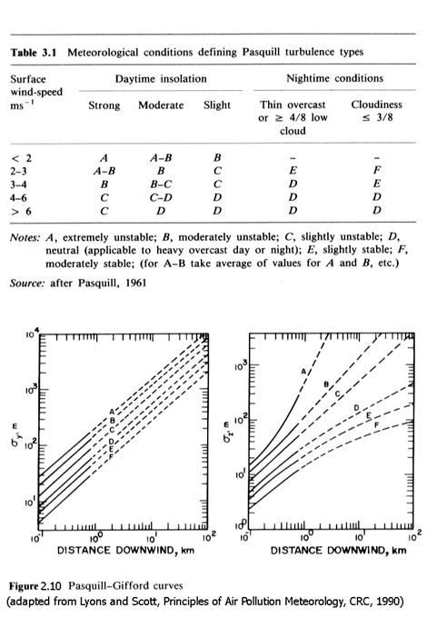
From experience, and the discussion above, we know that a smoke plume expands in both the y and z directions as it goes down wind. The expansion of the plume also depends on the air’s stability. Under very stable conditions, the plume will hardly expand at all, while under very turbulent conditions, it can expand rapidly. Considerable effort has gone into defining expressions that capture the relationships between s_y and s_z as a function of parameters that define stability and downwind distance. We present two of them, both based on the Pasquill turbulence types, as represented in Table 3.1. The different types are expressed as A, B, C, D, E, and F, and depend on the solar insolation and the wind speed. Once the proper type is identified, then s_y and s_z can be determined either from Figure 2.10, which is based on work by Pasquill and Gifford, or by the equations given by Briggs in Table 2.3.

Table 2.3. Briggs recommendations for s_y and s_z for 100 m < x < 10,000 m
Pasquill type	s_y(m)	s_z(m)
rural environments
A	0.22 x (1 + 0.0001 x)^-1/2	0.20 x
B	0.16 x (1 + 0.0001 x)^-1/2	0.12 x
C	0.11 x (1 + 0.0001 x)^-1/2	0.08 x (1 + 0.0002 x)^-1/2
D	0.08 x (1 + 0.0001 x)^-1/2	0.06 x (1 + 0.0015 x)^-1/2
E	0.06 x (1 + 0.0001 x)^-1/2	0.03 x (1 + 0.0003 x)^-1
F	0.04 x (1 + 0.0001 x)^-1/2	0.016 x (1 + 0.0003 x)^-1

urban environments
A-B	0.32 x (1 + 0.0004 x)^-1/2	0.24 x (1 + 0.001 x)^1/2
C	0.22 x (1 + 0.0004 x)^-1/2	0.20 x
D	0.16 x (1 + 0.0004 x)^-1/2	0.14 x (1 + 0.0003 x)^-1/2
E-F	0.11 x (1 + 0.0004 x)^-1/2	0.08 x (1 + 0.0015 x)^-1/2

For example, suppose it is noon in a sunny summer day, with the wind speed of 3-4 m s^-1. This condition corresponds to Pasquill turbulence type B. Therefore, from the curves in Figure 2.10, for x = 1000 m, s_y ~ 200 m and s_z ~ 100 m. From the Briggs formulae, s_y ~ 210 m and s_z ~ 120 m.

Problem 2.3. Dispersion in a Gaussian plume. Using the Pasquill turbulence types and the Briggs formulae, estimate the Gaussian plume expansion for the conditions at 10 am, 3 pm, and 10 pm on Thursday, 18 September. Determine the Gaussian equation and get the expansion at 1 km. You can get the wind speed at: http://www.srh.noaa.gov/data/forecasts/PAZ019.php?warnzone=paz019&warncounty=pac027 . Explain why you chose the Pasquill turbulence types that you did for the three different times.

The Gaussian plume model has long been used because of its simplicity and reasonable accuracy. The form given above is for the simplest case. We need to modify this expression for cases in which the pollutant hits the ground. The modified form depends on what happens to the pollutant when it hits. These cases include total reflection (bounces off), total absorption, and partial absorption.

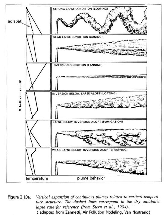
Remember that the Gaussian plume model applies to averages. There are clearly cases in which the instantaneous concentration of the plume’s constituents can be much greater at any point, as is illustrated in Figure 2.10a.

2.1 Trace chemicals

Trace chemicals are those atmospheric constituents that exist in the atmosphere at mixing ratios of a few ppm or less. They range from methane and stratospheric ozone, which are present in a few ppmv, to highly reactive constituents like the hydroxyl radical, OH, which is present at 0.02-1 pptv. Hundreds on chemicals exist in the atmosphere at the pptv to ppbv levels. Some are toxic; some are carcinogenic; some are harmless. Some play a large role in atmospheric chemistry; others play almost no role at all. The origin of essentially all trace atmospheric constituents is activity at Earth’s surface or atmospheric chemistry.

2.1.1 Families

Atmospheric constituents that have similar roles in atmospheric chemistry or that contain a particular type of atom, which, by its number of electrons, react in certain ways, are lumped together in chemical families.

The main chemical families involved with atmospheric chemistry are:

sulfur-containing compounds
nitrogen-containing compounds
carbon-containing compounds ( a very large group!)
halogen-containing compounds
hydrogen and oxygen compounds
oxygen only compounds (O₃, O, and O₂)

There is mixing across these lists – particularly with carbon – so that many molecules contain elements of different chemical families. Considering the functional behavior of that constituent for a given atmospheric condition, in addition to the molecules elemental components helps determine to which family a molecule belongs. For instance, often we are interested in budgets, that is, an accounting of the amount of a particular element in different molecules or even different reservoirs, such as the atmosphere, the oceans, the biomass, and the soil or rock. We can also be interested in the distribution of an element in different atmospheric molecules. An example of both of these types of budgets is the element nitrogen, N. Knowing how much nitrogen is released and removed from the atmosphere each year and how much is taken up by plants and the oceans is an important question that affects the behavior of several ecosystems. Often, knowing the distribution of nitrogen among its atmospheric forms can tell us about its sources and the chemical transformations that have occurred since it entered the atmosphere.

Every chemical emitted into the atmosphere eventually mostly ends up back on the surface (He is an exception). This entire process is called the biogeochemical cycle of the element.

I like Seinfeld’s definition of air pollution: “A condition of “air pollution” may be defined as a situation in which substances that result from anthropogenic activities are present at concentrations sufficiently high above their normal levels so to produce a measurable effect on humans, animals, vegetation, or materials.”

Although air pollution has long been a health problem, episodes in London in 1952 were so severe that over 4000 people died from breathing the air. In this case, the cause was the sulfur in the coal, which when burned, released SO₂ into the atmosphere. These episodes caused Britain to pass a Clean Air Act.

In the United States in 1944, Los Angeles vegetable crops were observed to be suffering damage. In 1951, this damage was shown to be from ozone. These studies were the beginning of attempts to understand photochemical air pollution from a scientific view.

Photochemical smog is now observed and studied world-wide.

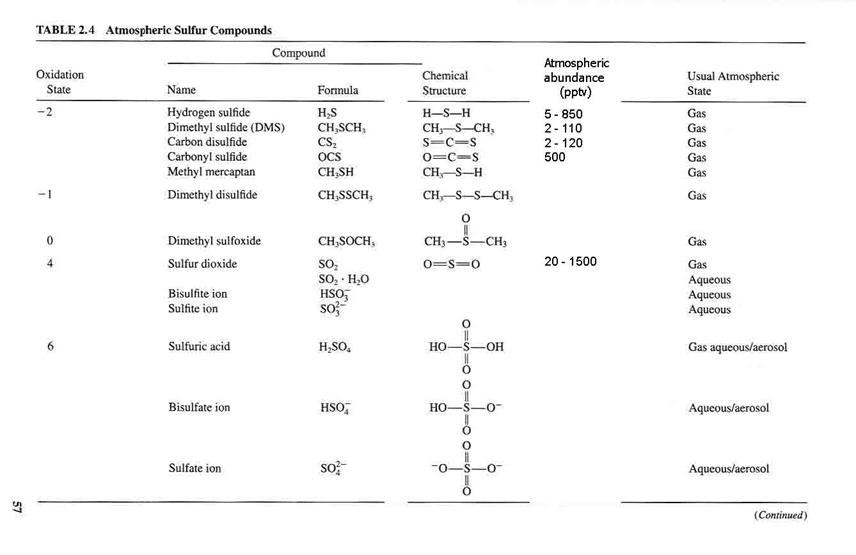
Sulfur-containing compounds.

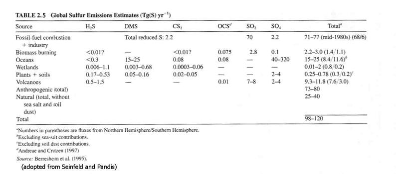
Table 2.4 contains the main sulfur atmospheric constituents.

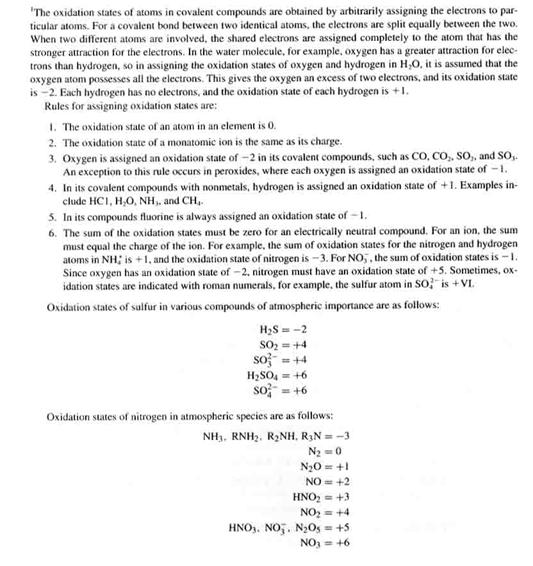
A brief discussion of oxidation states. The reason that this is notable is that we have an oxidizing atmosphere, in which compounds usually go from less oxidized (lower oxidation state) to more oxidized (high oxidation state). This discussion is on page 56 of Seinfeld and Pandis.

Note that anthropogenic sulfur emissions account for about 75% of all global sulfur emissions and that 90% of them are in the Northern Hemisphere.

See Table 2.5 for the main sulfur compounds and their sources.

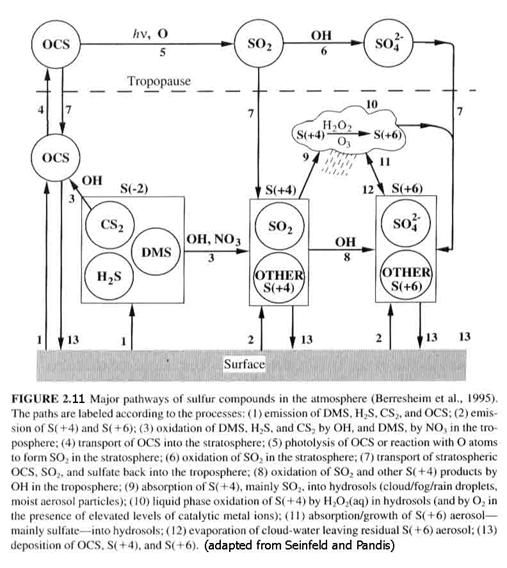
See Figure 2.11 for the atmospheric sulfur cycle.

Nitrogen-containing chemical family.

N₂ is the most abundant atmospheric nitrogen compound. However, its only role in atmospheric chemistry is that it supplies the nitrogen, by combustion or biological activity (nitrogen fixation = conversion of Nin N₂ to another compound), to compounds that are active in atmospheric chemistry. These compounds are:

nitrous oxide (N₂O), nitric oxide (NO), nitrogen dioxide (NO₂), nitric acid (HNO₃), and ammonia (NH₃). We will get to more minor players in a minute.

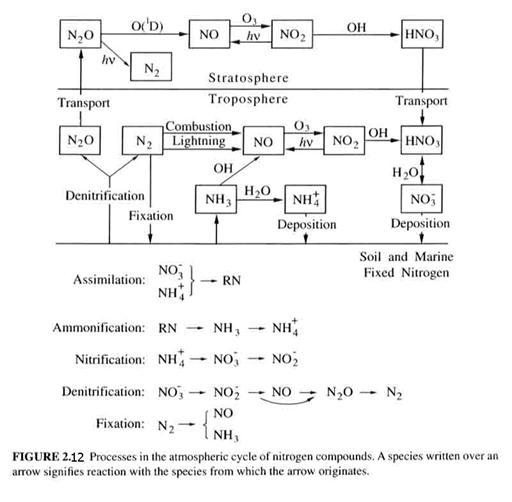
The biogeochemical cycles of nitrogen compounds can be seen in Figure 2.12.

Nitrous oxide (N₂O) is produced by biological activity. It is a powerful greenhouse gas and is inert in the troposphere. In the stratosphere, it is broken down by sunlight (90%), but the 10% that reacts forms most of the reactive nitrogen in the stratosphere. It’s atmospheric lifetime is about 120 years. It is well-mixed in the troposphere, with a value of about 315 ppbv.

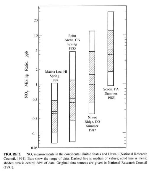
Nitrogen oxides. (NO and NO₂ = NO_x). These are two of the most important compounds in atmospheric chemistry. Their sources are given in Table 2.6. Table 2.7 shows that the mixing ratios for NO_x vary wildly, depending on the environment.

Nitric acid (HNO₃). Nitric acid is the major oxidation products of NO_x. Dry and wet deposition of HNO₃ are the major mechanisms by which NO_x is removed from the atmosphere.

Nitrates. Nitrates are chemicals that contain NO₃. There are many, although it is presently unclear as to how abundant most of them are. One important nitrate is peroxyacetyl nitrate (PAN), which has the chemical formula CH₃C(O)OONO₂. The O in “(O)” has a double bond to the carbon atom.

There are several other lesser compounds that we will talk about in more detail later. However, we are often interested in the total amount of oxidized nitrogen, and call this total NO_y.

NO_y = NO + NO₂ +HNO₃ + NO₃ + N₂O₅ + HONO + HO₂NO₂ + RONO + RONO₂ + RC(O)O₂NO₂ + …

Note that NH₃ is not included in NO_y. Values for NO_y are given in Figure 2.13.

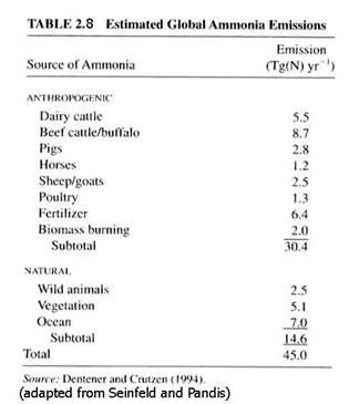
Ammonia (NH₃). An acid is a compound that is a electron acceptor in solution; a base is a compound that is an electron donor. NH₃ is the atmosphere’s primary basic gas. It has a number of sources and is easily absorbed in water and on surfaces. It is an important component of tropospheric aerosols because it can react with acids in the aerosol and neutralize them. The ammonia sources are given in Table 2.8. Note that anthropogenic sources make up a large part of the global ammonia production.

Carbon-containing chemical family.

Remember that carbon has 4 bonds. An organic compound is one that contains carbon.

Volatile Organic Compounds. VOCs include all gas-phase organic compounds, and thus not CO and CO₂. The atmospheric mixing ratios for VOCs range from pptv to ppbv levels generally, but can grow into the ppmv levels in polluted urban areas.

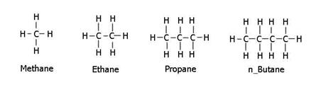
Alkanes. C_nH_2n+2. methane (CH₄); ethane (C₂H₆), propane (C₃H₈), n-butane (C₄H₁₀), …

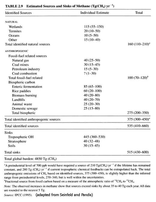
Methane. Methane is the atmosphere’s most abundant hydrocarbon, currently at 1745 ppbv. It has a huge flux through the atmosphere, as can be seen in Table 2.9. Methane’s lifetime is about 10 years. The methane concentration has more than doubled in the last 100 years, after being rather stable for the preceding millennium.

Alkanes react by hydrogen abstraction. This leaves a compound with an unpaired electron (called a free radical), which then can initiate other chemistry.

These free radicals are called alkyl radicals, and are often designated as “R”.

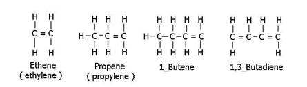
Alkenes. Alkenes have a double bond between some carbons. Ethene (CH₂=CH₂), Propene (propylene) CH₃CH=CH₂, etc. It is possible for molecules to have two double bonds, called alkadienes. Alkenes often react by addition of free radicals, also making an unstable compound.

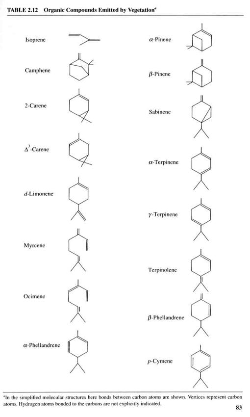
Trees and other plants emit a very reactive alkene called isoprene (C₅H₈). (Hence Ronald Reagan’s statement that “Trees pollute.”.) Isoprene is often present in mixing ratios of 1-10 ppbv in forested environments. Because of its reactivity with the hydroxyl radical, OH, it is one of the most reactive VOCs around. When the temperature rises, tree emit more isoprene. They also emit it during the day, but not at night. The exact reason that trees do this is not well known. See Figure 2.14. All except isoprene are aromatics, which will be discussed below.

Alkynes. alkynes have a triple bond. The best example is acetylene, HC≡CH.

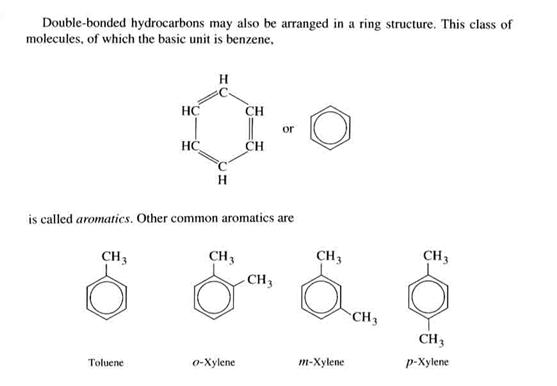
Aromatics. Double bonded hydrocarbons can be arranged as rings, such as benzene (C₆H₆). There are large numbers of aromatics in the atmosphere, some natural, some anthropogenic.

Polyaromatic hydrocarbons (PAHs). These compounds have more than one ring attached to each other. The simplest of these is naphthalene, which is two benzene rings joined together. Some anthropogenic PAHs are carcinogenic, although naphthalene is not one of those. Biogenic polyaromatic hydrocarbons are called terpenes. Monoterpenes consist of two rings joined together; sesquipterpenes consist of three rings joined together. Plants also emit large amounts of terpenes. Some emissions are both light and temperature sensitive, like isoprene; some are only temperature dependent, so that they are emitted both day and night.

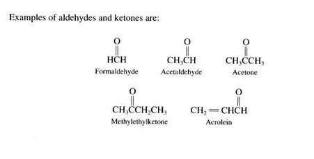
Oxygen-containing hydrocarbons = carbonyls.

aldehydes. The carbon is double-bonded to the oxygen., with an R and an H.

ketones. These have two alkyl groups.

Alcohols. Alcohols have an OH group attached. The simplest example is methanol (CH₃OH); another is ethyl alcohol (CH₃CH₂OH). These are another type of oxygenated hydrocarbons that have both biogenic and anthropogenic origins.

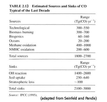
Carbon monoxide (CO). Table 2.13 gives the sources and sinks. CO is a product of incomplete combustion and atmospheric oxidation. On the global scale, CO is about 100 ppbv in the Northern Hemisphere and 50 ppbv in the Southern Hemisphere.

Halogen-containing chemical family.

Halocarbons is the general term for halogen-containing organic compounds.
chlorofluorcarbons (CFCs). They contain only carbon, fluorine, and chlorine and hard to break down in the atmosphere.
hydrochlorofluorocarbons. (HCFCs). contain hydrogen as well. – easier to break down in the atmosphere.
hydrofluorocarbons. contain hydrogen, fluorine, and carbon.
perhalocarbons. every available bond contains a halogen atom. CF₄.
Halons. bromine-containing halocarbons

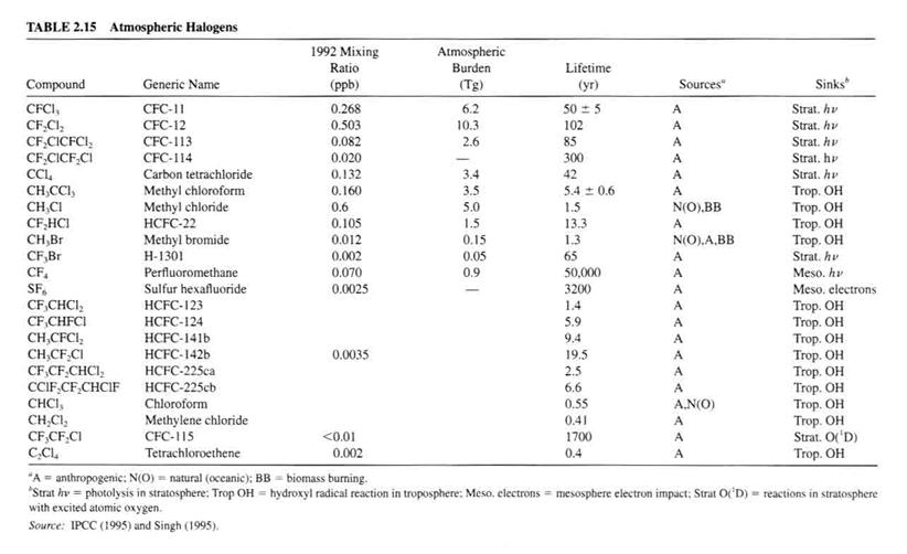
Table 2.15 lists some general halogen-containing compounds and their properties in the atmosphere.

Sulfur hexafluoride (SF₆) has special role. It has no known natural source and is used in transformers as a spark suppressant.

HCl. hydrogen chloride. This compound is emitted by volcanoes and is a product of atmospheric oxidation.

Organic halogen compounds: methyl chloride (CH₃Cl), methyl bromine (CH₃Br), … While methyl chloride is mostly natural, methyl bromine has both natural and anthropogenic sources, which are approximately equal. Methyl bromine kills small bugs and is used to fumigate the soil in the fields of commercial flower and fruit producers. It is also used to fumigate grain silos, and packing crates of produce being shipped into the United States.

Salts. Sea water contains large quantities of sodium chloride and sodium bromide. Heterogeneous reactions are capable of extracting Cl and Br, which then go on to create inorganic halogens that can participate in tropospheric chemistry. We will look at this chemistry in more detail later.

Ozone (O₃).

· The source of all ozone is photochemical. Because ozone is not emitted directly from the surface, it is sometimes called a secondary pollutant.

· 90% of O₃ is in the stratosphere; 10% is in the troposphere.

· Ozone absorbs ultraviolet light in the 290-320 nm region (UV-B).

· What is important is the total column of ozone between you and the sun. It does not matter if that ozone is in the stratosphere or the troposphere. What is important then is ozone’s column density, i.e., the ozone integrated over the path between the ground and the sun, per unit area. The units that are used are called Dobson Units (DU). 300 DU equals 3 mm of pure ozone at STP. 1 DU = 10^-3 atm cm.

· In the stratosphere, O₃ has mixing ratios of about 0.5 to 10 ppmv.

· In the troposphere, O₃ has mixing ratios of 0 to hundred’s of ppbv.

· Stratospheric ozone levels have been decreasing in the last 30 years. This allows more UV-B to reach Earth’s surface (1% O₃ decrease results in a ~2% increase in UV.) This increase influences tropospheric chemistry.

· Tropospheric ozone levels have increased in the last two hundred years, but it is unclear if they are increasing or decreasing at the present.

Particulate matter (aerosols).

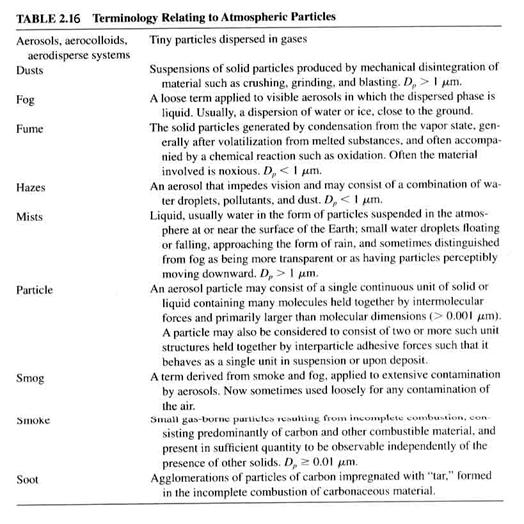
· Atmospheric particles take several forms, as in Table 2.16.

· Primary aerosols come directly from the surface or from emission sources; secondary aerosols are created from gas-to-particle conversion.

· Aerosol sizes range from nanometers to ten of microns.

· Small aerosols have concentrations of 10’s – several thousands cm^-3; large aerosols have concentrations of less than 1 cm^-3.

· Chemical composition includes: sulfate, ammonium, nitrate, sodium, chloride, trace metals, carbonaceous material (either elemental carbon – soot – or organic carbon), crustal elements, and water.

· Size of particle matter: <2.5 micron diameter, “fine”; > 2.5 micron diameter, “course”.

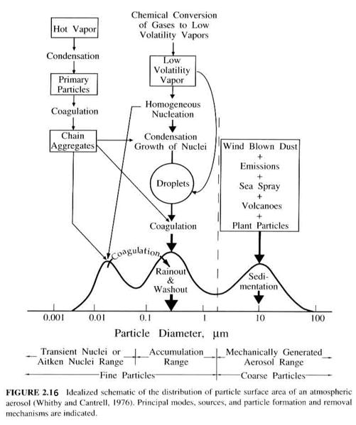
· Particles in the 0.005 to 0.1 mm are in the nuclei mode;

· Particles in the 0.1 to 2.5 mm diameter range are in the accumulation mode. (Figure 2.16)

Aerosols will be considered in much greater detail later.

2.3.4 Changes since pre-industrial times.

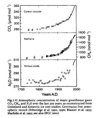
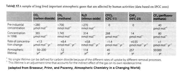
With the increase in population and industrialization has come rather significant changes to the atmospheric abundances of trace constituents. Background ozone appears to have roughly doubled or tripled, from 10-20 ppbv to 40 ppbv in the last 150 years. Other atmospheric trace constituents have changed as well, as shown in Figure 2.17 and Table 2.17. We see a rapid growth in atmospheric CO₂, CH₄, and N₂O. Understanding the details of these changes requires a good understanding of the sources and sinks of these atmospheric constituents.

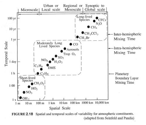
This chapter has introduced you to the atmospheric environment and its meteorology, which is typically thought to be little influenced by atmospheric chemistry and trace atmospheric constituents. It has also introduced you to the main atmospheric trace constituents that participate in atmospheric chemistry. One of the most important messages from this chapter is that chemical processes and transport processes both operate on a wide range of temporal and spatial scales (Figure 2.18). We must be very careful to not ignore transport processes when they occur on the same time scales as the chemical processes of interest. This is why chemical transport models (CTMs) have become so popular for examining atmospheric chemistry processes and for predicting and forecasting “chemical weather”.

Next, will be a brief discussion of the fundamental concepts of atmospheric chemistry. With knowledge of the atmosphere’s constituents and the fundamentals, we will be able to tackle the issues in atmospheric chemistry.