The Long-Term Carbon Cycle
Introduction
Earlier in this chapter, we designed and experimented with models of the global carbon cycle that are intended to simulate the short-term dynamics of the system. Here, short-term means a few hundred years, which is the briefest instant of time when seen in the context of the 4.6 billion years of Earth's history. We learned, among other things, that the system moves toward a steady state, with a response time of about 300 years or so. This means that, if left alone, the system would stabilize quickly enough so that on a geological timescale, it would appear to always be in a steady state. But, what if there are some slow changes that operate on much longer time scales of millions of years? Such changes could produce a sort of steady shift in the whole carbon cycle, but the system may appear to be in a steady state at any one point in time.
Gradual changes in plate tectonics may lead to gradual, long-term changes in the rate of volcanic/metamorphic emissions of CO2, uplift related to mountain-building may lead to changes in the global weathering rate, or changes in seal level may affect carbonate deposition, global weathering, and/or the nutrient supply to the oceans and thus the strength of the "biologic pump". These are a few examples of the kinds of changes in the carbon cycle that occur on longer time scales. Our goal in this section is to learn more about the general behavior of the carbon cycle on longer time scales by constructing and experimenting with a series of simple models.
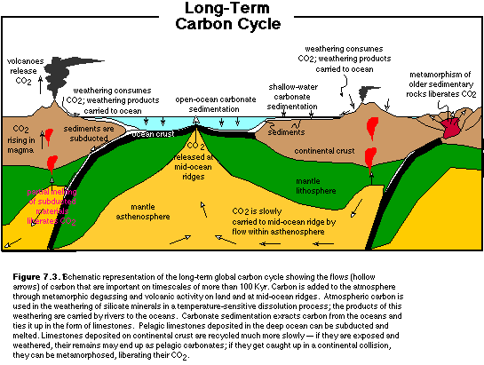
Figure 7.3.1 below shows some of the major processes and reservoirs that are important in the long-term behavior of the carbon cycle.

Processes and Relationships in Long-Term Carbon Cycle
Before constructing the model, we need to explore some of the more important processes involved in the long-term carbon cycle. The processes of interest are those that effectively are related to very long response times; the weathering of rocks exposed on land (and subsequent transfer of carbon via runoff to the oceans), sedimentation and burial of carbonate on the seafloor, and the release of CO2 through metamorphism and volcanism.
Weathering
If you recall from the first chapter of this book, the chemical weathering of minerals exposed at the surface is a seemingly benign, but potentially very important process. It is worth reiterating that what we're interested in here is not the weathering of limestones, but the weathering reactions involving silicate minerals. Although the weathering of limestones does indeed involve the transfer of carbon, it has no net effect on the amount of CO2 in the atmosphere.
We can review the general process of weathering silicate minerals by studying the following chemical reactions, paying particular attention to CO2:
(1) CaSiO3 + 3H2O + 2CO2 Æ Ca2+ + 2(HCO3- ) + H4SiO4wollastonite + water + carbon dioxide Æ calcium + bicarbonate + silicic acid
Here, the reactants (things on the left side) include a silicate mineral, water and carbon dioxide, the latter two coming from pore spaces in the soil, right near the surface. The carbon dioxide used here can be thought of as coming almost directly from the atmosphere since it is part of the rapidly recycling terrestrial portion of the carbon cycle. The products of this reaction are all carried away in solution, ending up in the oceans. The silicic acid will eventually be used by siliceous planktonic organisms; the calcium and bicarbonate ions will be combined by other organisms in the oceans, forming calcite and some dissolved carbon dioxide, which can escape back to the atmosphere:
(2) Ca2+ + 2(HCO3- ) Æ CaCO3 + H2O + CO2 �
Note that only one of the CO2 molecules is returned to the atmosphere in this step; the other is sequestered in the form of limestone (CaCO3).
The limestone has a choice of 3 different fates: 1) limestones deposited in very shallow water settings can be exposed by a small drop in sea level and thus undergo chemical weathering; 2) limestones deposited along a continental margin can be deeply buried and then metamorphosed during a continent-continent collision; and 3) limestones deposited on the deep ocean floor may get subducted and then melted. The first fate has no net effect on the carbon cycle, but the latter two both can release carbon dioxide to the atmosphere, thus closing the loop. The metamorphic reaction involved here is one that occurs when the calcite in limestone is intimately mixed with some quartz:
(3) CaCO3 + SiO2 Æ CaSiO3 + CO2 �calcite + quartz Æ wollastonite + carbon dioxide
Like melting, the metamorphism releases CO2 as a gas. So, the two molecules that were used in the silicate weathering at the outset are returned, completing the cycle. In reality, this is a relatively slow cycle, and it has some slow leaks in it, so that limestones have been accumulating over time.
The weathering reaction (1) above represents an important negative feedback mechanism in the long-term carbon cycle. Like most chemical reactions, the process of dissolution described in equation (1) above is sensitive to the temperature; the hotter it is, the faster the dissolution. Thus, if the climate is warm (high atmospheric CO2 ) then weathering will occur faster, removing CO2 from the atmosphere, cooling the climate. This negative feedback mechanism is potentially one of the most important long-term stabilizers in Earth's climate system.
Our formulation of the weathering flow will involve multiplying the estimated present day value for this flow by some function that represents the temperature-sensitivity of the weathering process. This function has been estimated from some laboratory experiments, and while it is better than nothing, we have to recognize that ideally, we would have a some good field-based experiments to guide our formulation. That said, the formula we use here is:
Here, Fw is the weathering flux, Fw,0 is the flux at the present day, T is the temperature at any time during experiment, and T0 is the present day temperature in °C. This equation defines a relationship that is shown graphically in the figure below:
Relationship Between Atmospheric Carbon and Global Temperature
We also need a way to keep track of the temperature in our model. In the other carbon cycle models, we basically used a simple linear relationship between CO2 concentration and temperature; this is fine for relatively small changes in CO2, but it is not appropriate for larger changes. In an earlier chapter, we saw how the effect of atmospheric CO2 on greenhouse warming diminished as the total CO2 concentration grew higher. Theoretical calculations (from Volk, see below) of this relationship provide us with a formula that we will use here:
Here, DT is the change in temperature, in °C, Matm is the amount of carbon in the atmosphere at any time, and Matm,0 is the starting amount. This equation is shown graphically below:
Sedimentation
Carbon is removed from the oceanic reservoir through the process of sedimentation of organic remains and inorganic carbonate shell material. Much of the inorganic carbon is ultimately recycled by bacteria in the ocean water or in the sediments on the sea floor, so most of the net removal of carbon occurs in the form of carbonate. This carbonate is produced almost exclusively by organisms, either open-ocean dwelling plankton (pelagic limestones), or bottom-dwelling creatures inhabiting warm, clear, shallow, tropical seas (continental shelf limestones). Pelagic limestones deposited on oceanic crust do not stick around for too long (200 Myr or less) due to subduction, whereas continental shelf limestones tend to have a much greater residence time. In this simple model, hoevere, we will not try to differentiate between these two types of limestone.
The process of sedimentation is initially set up to be a very simple, draining function; the rate of carbon withdrawal (sedimentation) from the ocean is a function of the relative amount of carbon in the reservoir multiplied by the presumed starting value, which is set up to be equal to the weathering flux. In reality, this process is much more dependent on things like the area of warm, tropical, shallow seas, the types of carbonate-producing organisms in existence, the nutrient supply, etc., but we must remember that our goal here is very modest and we are not attempting to insert all of the relevant controls on this process into our model.
Melting and Metamorphism
Melting of limestone occurs in tectonically active zones, typically where two plates are converging and material from the surface is dragged down into a subduction zone. The melting releases CO2, which can either escape into the atmosphere through a volcano above the subduction zone, or much later, as a mid-ocean ridge, where mantle material rises to the surface and undergoes partial melting. Metamorphism of limestone, in the presence of quartz can also liberate CO2, and in this case, the gas makes it way to the surface dissolved in water until the water emerges at some kind of thermal spring.
Like the process of sedimentation, the combined processes of melting and metamorphism are represented as a simple draining flow, i.e., proportional to the relative amount of carbon stored in the limestone reservoir multiplied by a value equal to our presumed present day weathering flux. In addition, this flow is multiplied by a factor called the "tectonic pulse", which is initially set to 1 and thus has no influence. The tectonic pulse will be used during the initial experiments with the model to investigate how the system responds to changes in tectonic activity.
Constructing the Model
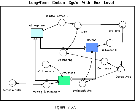
This model is very simple compared to the short-term models developed in the first part of this chapter. It consists of just three reservoirs representing the carbon in the atmosphere, the carbon in the ocean, and the carbon tied up in limestones. We leave out the mantle as a reservoir of carbon simply because of its vast size -- it is not likely to change significantly over the period of a few million years, which is the timescale we're looking at here. These reservoirs are connected by three flows -- weathering, sedimentation, and melting/metamorphism. Here, weathering represents the dissolution of silicate minerals, which uses CO2 from the atmosphere; sedimentation represents the formation and deposition of carbonate particles; and melting/metamorphism represents the liberation of CO2 from limestone deep within the Earth in tectonically-active zones (this also includes CO2 emitted from mid-ocean ridge volcanism, which really comes out of the mantle, but we're leaving the mantle reservoir out of this model).
The structure of this model is shown in in Figure 7.3.4 below, which, along with the accompanying equations, provide the necessary information to construct a working model of the long-term carbon cycle model.
Equations for Simple Long-Term Carbon Cycle
Experiments
Once you have constructed the model, run it for 2 million years (2 time units) with a time step of 0.005 and make sure that the model is in a steady state. This small DT is necessary because of the very small size of the atmospheric reservoir relative to the inputs and outputs.
1. Response Time of the System
A good first experiment that reveals a fundamental aspect of this system is one that changes the initial amount of a reservoir and then let's the model return to a steady state -- this defines the response time of the system. Set the initial value of the atmosphere reservoir to 1200 and then run the model long enough to determine the response time.
2. Changing Tectonic Activity
a) What will happen if there is a simple increase in the tectonic activity? There is an abundance of evidence suggesting that the tectonic activity of our planet undergoes change, so this is a relevant experiment to conduct. Change the Tectonic_Pulse graphic converter so that it has a value of 2 for the duration of the graph. The easiest way to do this is to click on the top of the Output column (thus selecting the whole thing) then typing 2 in the Edit Output box, then clicking on the OK button to exit. After making this change, predict what will happen, then run the model for 2 Myr and study the results. How good were your predictions? The change we've made is equivalent to saying that plate motions sped up by a factor of two, which is a dramatic change, but not so far-fetched, as we know from studies of spreading rates recorded by marine magnetic anomalies.
b) What will happen if there is a pulse in tectonic activity -- a brief increase followed by a return to the initial level? We can represent this quite easily since Tectonic_Pulse is set up as a graphical converter that changes over time. Simply insert a spike with a peak value of 2 at time=0.4 -- this will be a very short-lived increase in tectonic activity. Will the system return to its initial state, or will this tectonic pulse permanently change the system?
3. Exploring the Effect of Sea Level Changes
As the Earth's climate changes, so does the sea level due to the simple expansion and contraction of water upon heating and cooling, but also due to the build up or melting of glacial ice. In reality, sea level will also change as a function of the average age of the ocean crust, which in turn is a function of the rate of seafloor spreading, but this is a very slow form of sea level change and we will ignore it in this model. Changing sea level is important because it changes the areas covered by oceans and land and these areas in turn effect the global amount of carbonate sedimentation and weathering (greater surface area for weathering leads to a higher global weathering flux). To explore this effect, we need to make some changes to the model. First, we'll add a converter called Sea_Level and make a connector to it from Del_Temp, the converter that records the change in the global temperature. We'll make Sea_Level a graphical function of Del_Temp, using the following 13 pairs of data:
Then we'll make another new converter called Ocean_Area and define it as a graphical function of Sea_Level, using the following data, which come from a curve that shows the amount of Earth's surface plotted against elevation (called a hypsometric curve -- click here to see what it looks like) using the following 4 pairs of data:
We add one final new converter called Cont_Area, which will just be defined as:
Cont_Area = 1 - Ocean_Area
The next step is to make a connection from Cont_Area to weathering and another from Ocean_Area to sedimentation, redefining those flows so that they are multiplied by (Cont_Area/0.29) or (Ocean_Area/0.71) -- .29 and .71 are the starting areas of the continents and the oceans.
With these new changes, the model should look like this:

Now we are ready to do an experiment. Use the results from experiment 2a above as the control in this case, so make sure the Tectonic_Pulse converter is set to a value to 2 for the duration of the time. Before running the model, make a prediction about how this addition to the model will change its behavior.
References/Readings: