USING STELLA MODELS TO EXPLORE THE
DYNAMICS OF EARTH SYSTEMS
Dave Bice Department of Geosciences Penn Sate University University Park, PA 16802 dbice@geosc.psu.eduNote: This is a shortened version -- a more
thorough introduction to modeling systems with STELLA is also available.
What follows assumes that you have a copy of STELLA running on your computer,
along with the manual, which is very helpful and worth studying.
A First Modeling Exercise: The Water Tub
1. From the Real World to the Computer Model
2. Using the
model to illustrate systems concepts
The Purpose of Meaning of Computer Models
Some key concepts:
- steady state (dynamic equilibrium)
- residence time
- response time
- negative feedback mechanism
- positive feedback mechanism
- doubling time
- lag time
One of the most exciting recent developments in the earth sciences has been
the move towards looking at the Earth as a large, complex, interconnected system,
trying to understand how the system works. This field of study, earth system
science, is exciting not just because it is new (in fact, it is not that new --
see the appendix of Strahler and Strahler, 1989), but because it deals with
relevant issues such as global climate change and also because it is highly
integrative. In conversations with undergraduates at my college, societal
relevance and integration of different disciplines are, not surprisingly, some
of the things they are constantly looking for in their education. For these and
other reasons, earth system science is an attractive addition to many
undergraduate earth science courses.
But how does one go about teaching this material? Regardless of how you
choose to incorporate earth system science into geology classes, you face some
challenges associated with reviewing the relevant physics, chemistry, biology,
and meteorology that are needed to understand global systems such as the carbon
cycle. Another challenge arises when you search for ways to go beyond the
passive description of how various earth systems are constructed and how they
operate. Although dynamic systems surround us, we are not generally very good
at understanding and predicting their behavior without the aid of some type of model
that allows experimentation and observation. In this paper and a companion
paper, I describe -- in the form of several examples -- how computer models can
provide an effective means for enabling students to understand and explore the
dynamics of earth systems. This amounts to developing the systems part of earth
system science.
The task of using computer models to explore the dynamics of earth systems
is made much easier through the use of a program called STELLA (High
Performance Systems, Inc., http://www.hps-inc.com/) STELLA is essentially a
graphical programming environment that is specifically designed for modeling
systems that can be described by a series of differential equations. Users
construct graphical representations of systems and then enter values and
expressions corresponding to the components of the system. The program uses
this information to construct a set of differential equations that are
integrated over time used standard numerical techniques. STELLA runs on both
Macs and PCs.
It is important to note that although there is great value in developing the
programming skills and facility with differential equations needed to solve
these problems without the aid of a program like STELLA, it is nevertheless
possible to learn some important things about the dynamics of earth systems
without writing your own code. In fact, the algorithms used in STELLA are the
same used by most programmers to carry out numerical integration of
differential equations.
A First Modeling Exercise: The Water Tub
In order to illustrate some fundamental aspects of modeling and the behavior
of dynamic systems, I start with the simplest system imaginable -- a tub of
water with a faucet and drain.
1. From the Real World to the Computer Model
The first step in modeling is to define and consider the system as it
actually exists in the real world. This involves identifying the components of
the system, what material or entity is moving through the system, what
processes are involved moving this material or entity, and what kinds of things
these processes depend on. I find that this step is often facilitated by
drawing a cartoon of the system, as shown in Figure 1.
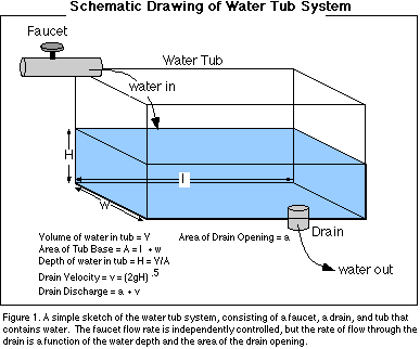
The faucet can be adjusted to supply water at whatever rate of flow we
choose. In contrast, the rate of flow through the drain is going to be a
function of the size of the drain opening and how much water is in the tub
because the weight of the water overlying the drain determines the amount of
pressure that is forcing the water through the drain. So, the outflow is
dependent on the amount of water in the tub. A more precise description of this
dependence is provided by Torricelli's Law, which states that the velocity of
water flowing out of a drain is equal to the square root of two times the
gravitational acceleration times the depth of the water above the drain. The
velocity is multiplied by the area of the drain opening to give an outflow in
volume of water per unit of time.
Figure 2 shows how this system is represented in STELLA; a box called a
reservoir represents the water tub, and two pipes called flows that represent
the faucet and the drain -- note that the flows have arrows on one side
indicating the direction of material transfer. The circles attached to the
flows represent valves that control the flow through the faucet and drain.
Another feature of this system are the thin arcuate arrows (connectors) that
represent some form of dependence or link between different parts of the system
-- for instance, the magnitude of the drain flow is dependent on the area of
the drain opening and the velocity of water flowing out the drain, which in turn
is dependent on the height of water in the tub, which in turn is dependent on
the amount of water in the tub. Below the reservoir are a set of circles called
converters that contain information on the details of the water tub and drain
opening -- some of these are simple constants, but those with connectors
leading to them are variables. Also note that the two flows have cloud symbols
at the ends away from the tub, indicating that this is an open system, drawing
water from some unspecified source, and sending it to an unspecified sink at
the other end.
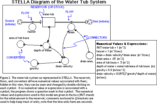
The model depicted in Figure 2 represents a complete model that is ready to
run after we specify the length of time (the time step, or dt of the
calculations) of the simulation and the increments of time over which the
program does the calculations. The user can also specify different integration
techniques, with the default being Euler's method. The time step is critically
important, and before any model results can be seriously considered, it is
important to try varying the time step to see how the model results change --
if the results do not change significantly, then the time step is at an
acceptable value; otherwise, the time step must be reduced to smaller values.
2. Using the model to illustrate systems concepts
There are a number of important concepts connected to dynamic systems that
can easily be illustrated with this simple model.
If we run the model for 100 seconds (Figure 3), we see some interesting
changes take place as the system evolves towards what is called a steady
state, or a dynamic equilibrium, where the amount in a reservoir stays constant
because the inflow and outflow are equal – in this condition, things are
changing and water is flowing, but the system as a whole is holding steady. The
inflow stays constant over time, but the outflow undergoes an exponential
change, increasing until it approaches the same value as the inflow. Initially,
the inflow is greater than the outflow, and so the amount of water, and
therefore the depth of the water in the tub increase, thus increasing the drain
velocity and the outflow; this continues until the inflow and outflow match, at
which point water continues to move through the system, but the amount of water
in the tub remains the same.
When the system is in the steady state, we can define another concept -- the
residence time. The
residence time is effectively the average length of time that an entity, in
this case a water molecule, remains in a reservoir. It is really only
meaningful for a reservoir that is at or near a steady state condition. By
definition, the residence time is the amount of material in the reservoir,
divided by either the inflow or the outflow
(they are equal when the reservoir is at steady state). If there are multiple
inflows or outflows, then we use the sum of the outflows or inflows to
determine the residence time. For our water tub system here, the residence time
is thus 10.16 m3 (the amount in the reservoir at the steady state condition)
divided by 1 m3/sec per second (the outflow at steady state), giving us 10.16
seconds for the residence time. It is fairly easy to see that if we increase
the flow rates, the water moves through the reservoir faster, so the residence
time decreases. It is possible then, to calculate any of the above three
parameters (residence time, reservoir amount, and inflow or outflow) if the
other two are known and if we assume the system is in a steady state. For
instance, if we assume that the human population is in a steady state (wishful
thinking), and if we know the average residence time, also known as the life
span, we can calculate the number of births and deaths in a year. The
population is close to 5.6 billion, so if we assume an average life span of 70
years, then we can say that 80 million people are born each year and 80 million
people die each year, assuming a steady state. Residence time is an important
concept in problems of pollutants in ground water or surface water reservoirs,
and also in understanding the long-term effects of greenhouse gases added to
the atmosphere.
A closely related concept is that of the response time of a system, which measures how quickly a
system recovers and returns to its steady state after some perturbation. We can illustrate this concept by running several
simulations, where we vary the starting amount of water in the reservoir and
pay attention to how quickly the system gets to its steady state. The results
are shown in Figure 4.
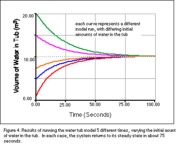
It may come as somewhat of a surprise to see that regardless of how great
the initial departure from the ending steady state, this system gets to the
steady state at about the same time. In an even simpler system, where the
outflow (D) is defined as a simple fraction (k) of the amount in the reservoir
(W) such that at each instant in time, D = kW, the response time is defined as
1/k -- this turns out to be the time needed for the system to accomplish 63% of
the return to its steady state. Also note that in a very simple system, the
residence time and the response time are numerically the same even though they
are conceptually different. The response time is a very useful concept because
if it is known (or hypothesized), we can make some predictions about how
quickly the system will respond to a change in a reservoir. Alternatively, if
we change one of the inflow or outflow processes, we can predict how that will
affect the response time of the system.
A more detailed discussion of the concepts and mathematical formulation of
residence time and response time can be found in Rodhe (1992). Alternatively,
follow this link.
Another important observation to be made here is that the system evolves to
the same steady state in each case, so the steady state of a system (along with
the response time) is primarily determined by the nature of the inflows and
outflows.
This particular system we've been experimenting with returns
a steady state because it contains a negative feedback mechanism in the
connection between the drain flow rate and the amount of water in the tub. A negative
feedback mechanism is a controlling mechanism,
one that tends to counteract or diminish some kind of initial
imbalance or perturbation. A good example
of another negative feedback mechanism is a simple thermostat in a home that
responds to changes from the steady state, returning the home to a specified temperature.
Note that the word negative, as used here, does not mean that this is bad
feedback; it just means that this feedback mechanism acts to reverse the change
that set the feedback mechanism into operation. So if our tub is in its steady
state, knocking the system out of its steady state by suddenly dumping in more
water will cause a response -- the drain will increase its flow rate, thus
decreasing the amount of water in the tub, bringing back towards the steady
state value. If we instead decrease the amount in the tub, the negative
feedback associated with the drain forces the amount of water in the tub to
increase until the steady state is returned. The important thing to remember is
that negative feedback mechanisms tend to have stabilizing effects on systems.
In contrast, a positive feedback mechanism is one that exacerbates some initial
change from the steady state, leading to a runaway condition -- it acts to promote an enhancement of
the initial change. A simple way to modify
the simple water tub system in order to create a positive feedback system is to
alter the system as shown in Figure 5.
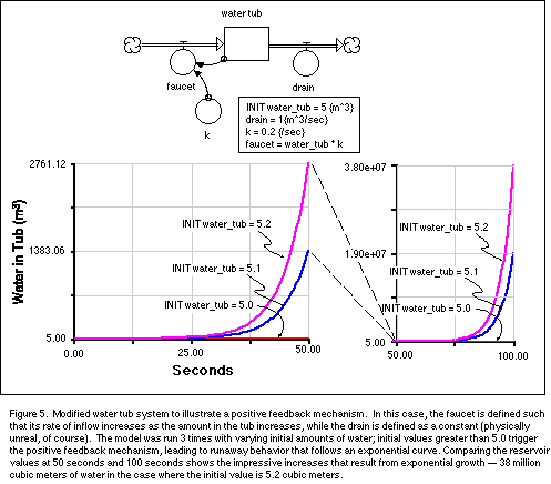
This system has one possible steady state, where the inital amount in the
water tub is 5 cubic meters; any departure from this value, however slight,
leads to runaway behavior and the amount of water in the tub follows an
exponential curve of the form:
![]()
where W(t) is the amount of water in the tub at any time, d is the drain
constant (1 in our case), k is the faucet rate constant (0.2), Wo is the initial amount of water in the tub
(variable in the 3 model runs shown in Fig. 5), and t is time. A useful thing
to remember with exponential growth is that the doubling
time (time required to increase the amount
in a reservoir by a factor of two) can be easily calculated (after some
manipulations of the above equation):
![]() .
.
Here, the doubling time works out to be 3.465 seconds.
If you run this model with an initial water tub value of less than 5, you
learn another important lesson, which is that in the real world, there are
limits to exponential change, regardless of whether that change leads to growth
or decline. In this case, the limit is reached when the there is no more water
left in the tub. In the case of population growth, the limit to exponential
growth is reached when the carrying capacity of the ecosystem is approached --
then the population growth decelerates and gradually approaches the carrying
capacity (with reference to the human population, see Cohen, 1995, for a
detailed discussion).
Positive feedback mechanisms, like negative feedback mechanisms are not
necessarily good or bad. Epidemics and infections have positive feedback
mechanisms associated with them, but so does the growth of money in a bank
account with compounded interest. The Earth contains a wide variety of both
positive feedbacks and negative feedbacks and depending on the conditions,
either kind of feedback may dominate. But, and this is very important, the mere
fact that we exist, the fact that our planet has water and an atmosphere is
compelling evidence to suggest that ultimately, our Earth system is dominated
by negative feedback mechanisms (see Kasting, 1989 or Lovelock, 1988 for more
on this). In addition, it is equally important to realize that human time
scales are much shorter than the history of the Earth and over periods of time
that interest humans, positive feedback mechanisms may be very important; they
have the potential to produce dramatic changes.
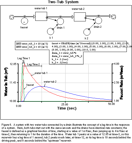
We next consider a slightly more complex system to illustrate the concept of
a lag time – the time difference in the response of
different parts of a connected system (best seen graphically below). In Figure 6, two water tubs have been connected
such that the drain from one flows into the adjacent tub. Here, the drains have
been simplified greatly -- all of the drain parameters in our first model are
represented by a rate constants labeled k1 and k2; these rate constants get multiplied
by the amount in the reservoir at any time to give the volumetric rate of flow
out of the drain. Next, we take advantage of a useful feature of STELLA -- the
ability to define various parameters as graphical functions of other system
variables or time. In this case, I want to show how the system responds to a
sudden spike in the faucet flow rate, so I first define the faucet rate as
being equal to time, then click on a button in the dialog box and a graph
appears, enabling you to define the nature of this graphical relationship. The
faucet in this case starts out with a value of 1 m3/sec, which puts the system
in a steady state to begin with, then increases to a peak value of 4, and then
quickly returns to 1 again and stays there for the duration of the experiment.
The response of the system is shown in Figure 6. The first tub reaches its
peak 1 second behind the peak in the faucet -- it lags behind the faucet. The
second tub peaks at a lower value and much later than the first -- the
perturbation is buffered by the first water tub. Note that both tubs return to
their steady state after variable amounts of time and that the total area under
the two curves is equal, meaning that the same volume of water moved through
each reservoir. The pulse of extra water, propagating through the system is
very similar to the pulse of water moving down a stream system, with the lag
time in this analogy being the time between the peak in the rainfall and the
flood peak along a certain reach of the stream. The concept of a lag time is
also relevant to systems such as the global carbon cycle -- anthropogenic
additions of CO2 into the atmosphere are similar to the faucet here; the
climatic response involves a certain lag time. This lag time means that if we
halt emissions today, the climate will continue to warm -- a fact that may
policy-makers and citizens should be aware of.
The Purpose of Meaning of Computer Models
Modeling is an important part of science and has grown in pace with the
increased availability of computing power. Many models deal with systems that are
of great societal importance (e.g., global warming, el Niño events), making it
increasingly important to understand the process, goals, and limitations of
models. This understanding is essential for intelligent interpretation of model
results.
The purpose of a model is not to replicate the real world -- it is clearly
impossible to put the complexity of the real world into a computer. Instead,
the goal is usually to understand something about the behavior of systems and
also to understand the affects of changes on the system -- its response to
changes. We create and use these models because their real-life versions are so
complex and large that we cannot generally understand them without some kind of
controlled experimentation.
The meaning and significance of model results depends largely on the intent
of the model and whether the model captures the essence of the real-world
system. Many models, including the ones shown here, do not include mathematical
expressions that are detailed enough, incorporating all of the physics of the
relevant processes to generate results that are quantitatively precise over a
wide range of conditions. In most models, the goal is to create a model that
incorporates our best approximation of the important components, processes, and
relationships that make up a system. This inevitably means finding relatively
simple mathematical expressions for complex processes, often relying on
observations of the process to create empirical, mathematical descriptions -- a
nice example of this is Torricelli's Law used in the model above. A model
constructed in this manner allows us to explore the implications of our
assumptions that went into the model, focusing on the qualitative aspects of
the results more than the actual numbers.
The next question is: How do we evaluate the results of a model in relation
to the real world? In the case of our water tub model, the answer is simple --
construct a real version of the model and collect some real data and then see
if the computer model can reproduce the results. If this succeeds, then we can
conclude that our model captures the essence of the system; if not, then we
must examine the model carefully, make revisions, and then re-test.
The process of constructing a model inevitably raises new questions and
encourages further consideration and possibly new research into the processes
involved in the system. Thus, the process of model construction is itself a
process of learning and inquiry that is beneficial even if the model never
evolves to the point of passing all the real world tests.
- Cohen, J.E., 1995, How many people can the Earth support?, New York, Norton, 532 p.
- Kasting, J., 1989, Long-term stability of the Earth's climate, Global and Planetary Change, v. 1, p. 83-97.
- Lovelock, J., 1988, The Ages of Gaia, New York, Norton, 325 p.
- Rodhe, H., Modeling Biogeochemical Cycles, in, Butcher, S.S., Charlson, R.J., Orians, G.H., and Wolfe, G. V., (eds.) Global Biogeochemical Cycles, Sand Diego, Academic Press, 379 p.
- Strahler, A.N., and Strahler, A.H., Physical Geography, 4th Ed., New York, John Wiley and Sons, 562 p.