There are probably an infinite number of models of dynamics
systems, but some common design elements or system structures are
found in a great number of models. When we venture off into world of
modeling, it will be helpful to be familiar with some of these common
designs and it will be especially helpful develop a sense of what
types of behaviors are associated with these designs.
The series of figures below illustrate these comon system designs
in the form of very simple STELLA models, accompanied by graphs that
show the behavior or evolution of these systems over time, and the
basic equations used in the models. In each case, I mention a
real-life system that similar to these models.
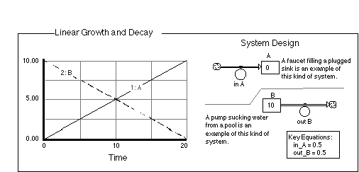
Figure 2.14 Linear Growth and
Decay. The key to this system design is that the flows are defined as
constants; this results in a very simple, easy-to-predict behavior
characterized by constant rates of change.
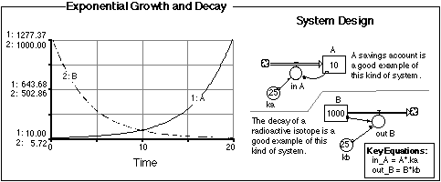
Figure 2.15 Exponential Growth
and Decay. These are extremely common design elements that are
sometimes referred to as first-order kinetic equations, but in
simpler terms, they represent growth or decay (draining) processes
where the rate of change is a fixed percentage of the reservoir
involved in the flow. Exponential growth represents a classic form of
positive feedback, yielding a runaway behavior, while exponential
decay represents a negative feedback mechanisms that has a
stabilizing effect.
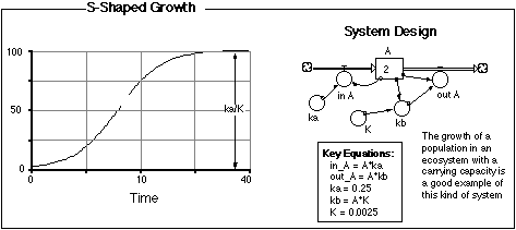
Figure 2.16 S-Shaped Growth. This
system design is especially common in models of population growth
that is limited by some resource. In this type of a system, one of
the flows is defined as a percentage of the reservoir, but that
percentage changes as the amount in the reservoir changes. This kind
of a system design has a sort of built-in limit, determined by the
rate constants, as shown in the figure. Interestingly, this sytem
structure can lead to chaotic behavior as we will see in a later
chapter on population growth.
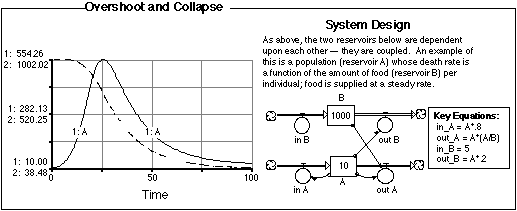
Figure 2.17 Overshoot and
Collapse. This system design represents a variation on the system
shown in Figure 2.16. In this case, the limit to growth, represented
by reservoir B is declining as reservoir A increases. Reservoir A
grows exponentially and shoots past its limit and as a result, the
limit decreases more and more, fueling a collapse of A until it
reaches a steady-state at a very low level.
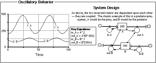
Figure 2.18 Oscillatory Behavior.
This type of system design represents what is called a coupled system
since the change of each reservoir is dependent on how its companion
reservoir is changing. These systems often lead to an oscillation,
creating cycles that do not have an external control. The oscillation
arising from these coupled reservoirs is very different from the kind
of oscillation forced onto a system by some external control -
something that is a sinusoidal function of time.
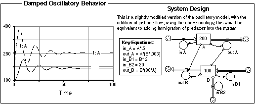
Figure 2.19 Damped Oscillatory
Behavior. This is a variation of the system shown in Figure 2.18 and
is common in any environment where friction or some other form of
energy loss is a factor. Interestingly, it is also a consequence of
migrations in systems of coupled populations.
RETURN TO MAIN PAGE