To embark on our modeling adventures, let's begin with a very
simple example of a dynamic system - one involving the flow of water
in and out of a bathtub. This may not seem too glamorous, but the
bathtub is a classic example that most people can relate to with some
degree of fondness. The bathtub model will provide a good foundation
for investigating more complex models that are more directly related
to the global climate system.
Introduction to the Bathtub System
First, a sketch of what this system might look like, for those of you who only take showers:
We have an ordinary tub with a faucet pouring water into the tub
and a drain that allows water to flow out of the tub. The faucet is
assumed to tap into an infinite source of water; likewise, the drain
removes water beyond the confines of the system. You can see that
this is an open system rather
than a closed system - the ultimate sources and sinks of water
are beyond the confines of the system; we're not keeping track of
them.
The faucet can be adjusted to supply water at whatever rate of
flow we choose. In contrast, the rate of flow through the drain is a
function of the size of the drain opening and how much water is in
the tub because the weight of the water overlying the drain
determines the amount of pressure that is forcing the water through
the drain. So, for a given drain size, the more water in the tub, the
greater the rate of flow. This set-up we've just described is a
dynamic system because material is flowing through the system and the
rates of flow and the amount of water in the tub are likely to change
over time.
Systems Diagram of the Watertub
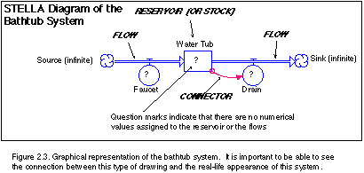
Next, we'll represent this system in a different form - a
graphical diagram that was created in the program STELLA. The figure
below shows the STELLA diagram of this system, consisting of a box
called a reservoir (or stock) that represents the water tub, and two
pipes called flows that represent the faucet and the drain. Note that
the flows have circles attached - these represent valves that control
the flow through the faucet and drain. The other feature of this
system is an arrow that connects the water tub reservoir to the drain
outflow - this is called a connector in STELLA terminology and
represents the fact that the rate of flow through the drain is
somehow dependent on the amount of water in the reservoir. Note that
no material flows through this arrow, instead, it represents a kind
of information transfer - the drain flow rate gets information from
the reservoir. Also note that the two flows have cloud symbols at the
ends away from the tub, indicating that this is an open system,
drawing water from some unspecified source, and sending it to an
unspecified sink at the other end.

Constructing a STELLA Model of the System
At this point, you should start up the program STELLA and follow
along with the instructions below as we create and manipulate the
bathtub model. It is possible to follow along without using the
program, but it is a good idea to begin getting some experience
working with the program.
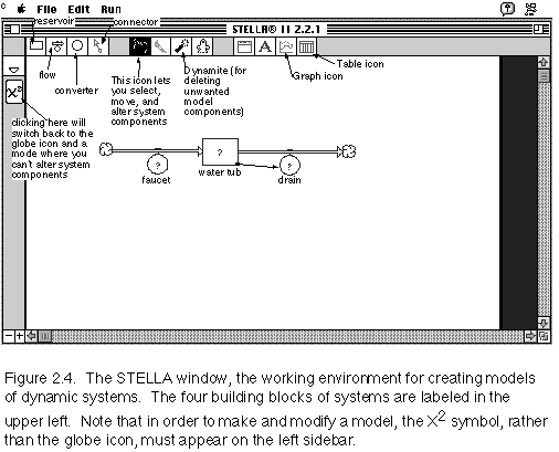
As with all Macintosh programs, the first step is to double-click
on the program icon. When the program first starts. you should see a
window like that shown below, in Figure 2.4. If you don't see this
same window (minus the comments, of course), you must click on the
icons that appear along the left sidebar until the
X2 icon appears - then you are in the working
mode of the program (the other modes are for viewing the equations or
just looking at the model without making any changes).

To create the model of the bathtub, first select the reservoir
tool, then move the cursor to the middle of the window, and click on
the mouse button to deposit a reservoir. Then, select the flow tool,
move the cursor down into the window, positioning it slightly to the
left of the reservoir; click and hold the mouse button and drag the
cursor into the middle of the reservoir and release the mouse button,
making the connection. A cloud symbol should appear on the left side
of this flow. Select the flow tool again and position the cursor in
the middle of the reservoir before clicking the mouse button. As
before, click, hold, and drag the cursor to the right and then let up
on the mouse button. The next step is to select the connector tool
and position the cursor in the middle of the reservoir and then
click, hold, and drag until the arrow tip is in the middle of the
circle attached to the drain flow, then release the mouse button and
the connection should be made. When you've completed these steps,
select each system component by clicking on it and give it a label.
By this point, you should have a model that looks similar to the one
shown in Figure 2.4.
Note that at first, question marks appear in the reservoir and the two flows. This indicates that we have not assigned any kind of numerical quantity or mathematical expression to these system components. But by double-clicking on these various system components, we can add numbers and/or expressions to eliminate the question marks and make this a fully functional model. To begin with, we'll assign the following numbers or expressions to the system components:
Initial value for the Water Tub reservoir = 10.0 {liters};
Flow rate for the faucet = 1 {liter/second};
Flow rate for the drain = 0.1 * Water Tub {liters/second}.
Be sure to keep track of the units inside of the {} brackets -
losing track of the units is one of the most common causes of
problems with STELLA models. Note that by choosing liters per second
as the flow rate, we have effectively decided that our basic time
unit will be one second. All of these numbers are perfectly
arbitrary, and the expression for the drain flow rate is just a
simple relationship that says the drain flow rate is directly
proportional to the amount of water in the tub at any given time -
the quantity Water Tub can change through time. Once these values
have been assigned, our model is completed and is ready to "run". The
model "runs" through time, beginning at time=0 and going as long as
we specify. We can set the length of the run by selecting Time Specs
from the Run menu. Go ahead and select that command and set the
ending time to 60, with a time step or DT of 0.25. What is
this DT? It is the increment of time over which the program does the
calculations specified by the model, so it is one quarter of a second
in our case. This means that the program calculates how much water
enters and leaves the bathtub every quarter of a second. So if the
faucet flow rate is set to 1 liter/second, the program will add 0.25
liters every quarter of a second or DT. So the smaller the DT, the
more calculations are done. When the accounting is done in small
increments, the program generally does a better job of simulating the
real system. The time step, DT, is an important part of the program
to understand - we will have to pay attention to it as we begin
modeling the various parts of the climate system.
You may have noticed that in the same window where we set the
starting and ending time and the time step, there are many other
choices to be made. One of them concerns the units of time - this
controls what gets printed out on graphs that display the results of
simulations. You can also set the integration method, that the
program uses to make the calculations. It is not important that you
understand what this means at this point, but for future reference,
remember that Euler's method is usually the default method; it is the
fastest. The Runge-Kutta methods give more accurate results, but
cause the program to run more slowly. It is often a good idea to run
your models with a variety of DTs and integration methods to be sure
that your results are not an artifact of the calculation method.
Once you have set the time specs, the program is really ready to
run. We have two choices for how to observe the evolution of this
model - animation of the system components or graphs that plot the
values of various system components over time. The animations are not
as exciting as you might guess and they are not as informative as the
graphs, so we'll ignore them here. Before running the model, we need
to make a graph, so select the graph icon from the tool palette and
position the cursor somewhere convenient and click on the mouse
button to deposit the graph. The program then presents you with a
blank graph and you have to tell it what you want to plot by
selecting Define Graph from the Edit menu,
giving you a window with two columns at the top. Click on water
tub in the Allowable column, then click on the >> button
immediately to the right of the Allowable column, which moves
water tub over to the Selected column. Do the same for
faucet and drain so that you have all three in the
Selected column; click on the OK button at the bottom of this window
when you're finished. Now we are almost ready to run the model, but
not quite.
First, think about how this system might evolve - try to predict
how the amount of water in the tub, the faucet flow rate, and the
drain flow rate will change over time, given the equations listed
above. You might represent your prediction in the form of a graph,
similar to the one that the program will generate. Once you've made
your prediction, you are finally ready to run the model, so select
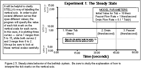
Run from the Run menu and see what happens. Your results should look
like the graph shown below in Figure 2.5.

How did you do? Were you able to predict how some or all of the
system components changed over time? As you can see (and as I'm sure
you all successfully predicted!), nothing changes in this system -
the flow rates and the amount in the reservoir are constant through
time, so the system is in a steady state. Water is still flowing
through this system, but the flow rates and volume in the reservoir
remain steady.