DICE Model Background

The global climate system and the global economic system are intertwined — warming will entail costs that will burden the economy, there are costs associated with reducing carbon emissions, and policy decisions about regulating emissions will affect the climate. These interconnections make for a complicated system — one that is difficult to predict and understand — thus the need for a model to help us make sense of how these interconnections might work out.
The economic model we will explore here is based on a model created by William Nordhaus of Yale University, who is considered by many to be the leading authority on the economics of climate change. His model is called DICE, for Dynamic, Integrated Climate and Economics model. It consists of many different parts and to fully understand the model and all of the logic within it is well beyond the scope of this class, but with a bit of background we can carry out some experiments with this model to explore the consequences of different policy options regarding the reduction of carbon emissions.
The DICE model includes a more primitive version of the global carbon cycle model we used earlier, but here, we will make some adaptations to our carbon cycle model so that it includes the economic components of DICE.
The economic components are shown in a highly simplified version of a STELLA model below:
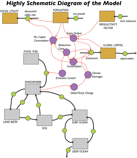
In this diagram, the gray boxes are reservoirs of carbon that represent in a very simple fashion our global carbon cycle model from Module 5; the black arrows with green circles in the middle are the flows between the reservoirs. The brown boxes are the reservoir components of the economic model, which include Global Capital, Productivity, Population, and something called Social Utility. The economic sector and the carbon sector are intertwined — the emission of fossil fuel carbon into the atmosphere is governed by the Emissions Control part of the economics model, and the Global Temp. Change part of the carbon cycle model affects the economic sector via the Climate Damage costs.
Let’s now have a look at the economic portions of the model.
The Global Capital Reservoir
In this model, Global Capital is a reservoir that represents all the goods and services of the global economic system; so this is much more than just money in the bank. This reservoir increases as a function of investments and decreases due to depreciation. Depreciation means that value is lost, and the model assumes a 10% depreciation per year; the 10% value comes from observations of rates of depreciation across the global economy in the past. The investment part is calculated as follows:
Investment = Savings Rate x (Gross Output - Abatement Costs – Climate Damages)
The savings rate is 18.5% per year (again based on observations). The Gross Output is the total economic output for each year, which depends on the global population, a productivity factor, and Global Capital.
Abatement Costs
The Abatement Costs are the costs of reducing carbon emissions, and are directly related to the amount by which we try to reduce carbon emissions. If we do nothing, the abatement costs are zero, but as we try to do more and more in terms of emissions reductions, the abatement costs go up. If we go all out in this department, the Abatement Costs can rise to be 15% of the Gross Output.
Climate Damages
Climate Damages are the costs associated with rising global temperatures. The way the model is set up, a 2°C increase in Global Temperature results in damages equal to 2.4% of Gross Output, but this rises to 9.6% for a temperature increase of 4°C, and 21.6% of Gross Output for a 6°C increase. This relationship between temperature change and damage involves temperature raised to an exponent that is initially set at 2, but can be adjusted.
Relative Climate Costs
It will be useful to have a way of comparing the climate costs, which is the sum of the Abatement Costs and the Climate Damages in a relative sense so that we see what the percentage of these costs is relative to the Gross Output of the economy. The model includes this relative measure of the climate costs as follows:
Relative Climate Costs = (Abatement Costs + Climate Damages)/Gross Output
Consumption
Also related to the Global Capital reservoir is a converter called Consumption. A central premise of most economic models is that consumption is good and more consumption is great. This sounds shallow, but it makes more sense if you realize that consumption can mean more than just using things it up; in this context, it can mean spending money on goods and services, and since services includes things like education, health care, infrastructure development, and basic research, you can see how more consumption of this kind can be equated with a better quality of life. So, perhaps it helps to think of consumption, or better, consumption per capita, as being one way to measure quality of life in the economic model, which provides a measure for the total value of consumed goods and services, which is defined as follows:
Consumption = (Gross Output – Climate Damages – Abatement Costs) – Investment
This is essentially what remains of the Gross Output after accounting for the damages related to climate change, abatement costs, and investment.
Population
The population in this model is highly constrained — it is not free to vary according to other parameters in the model. Instead, it starts at 6.5 billion people in the year 2000 and grows according to a net growth rate that steadily declines until it reaches 12 billion, at which point the population stabilizes. The declining rate of growth means that as time goes on, the rate of growth decreases, so we approach 12 billion very gradually.
Productivity Factor
The model assumes that our economic productivity will increase due to technological improvements, but the rate of increase will decrease, just like the rate of population growth. So the productivity keeps increasing, but it does not accelerate, which would lead to exponential growth in productivity. This decline in the rate of technological advances is once again something that is based on observations from the past.
Social Utility
The social utility reservoir is perhaps the hardest part of the model to understand. This reservoir is the accumulated sum of something called the social utility function, which depends on the size of the global population, the per capita (per person) consumption, and something Nordhaus calls the social time preference factor, which includes a discount rate and another parameter (alpha) that expresses society’s aversion to inequality.
The Discount Rate
One of the most obvious ways of addressing climate change is to reduce carbon emissions. This can be done by developing alternative energy sources, by capturing and sequestering carbon from power plants, by developing more efficient technologies, etc., but all of these cost money and they will continue to cost money into the future. How should we value those future costs at the present time?
The concept of a discount rate is an important one for this kind of economic modeling since it provides a way of translating future costs into present value. Here is how an economist might think about it: imagine you have a pig farm with 100 pigs, and the pigs increase at 5% per year by natural means. If you do nothing but sit back and watch the pigs do their thing, you’d have 105 pigs next year. So 105 pigs next year can be equated to 100 pigs in the present, with a 5% discount rate. Thus, the discount rate is kind of like the return on an investment. Now think about climate damages. If we assume that there is a 4% discount rate, then $1092 million in damages 100 years from now is $20 million in present day terms. It may seem odd to treat damages like this — they do not reproduce naturally like pigs — but it does make sense if you consider that our global economy is likely to grow quite a bit in 100 years, so that something worth $20 million today will be worth $1092 million in 100 years. The 4% figure is the estimated long-term market return on capital.
Why is this important? We would like to be able to see whether one policy for reducing emissions of carbon is economically better than another. Different policies will call for different histories of reductions, and to compare them, we need to sum up the expected future damages associated with each policy. The discount rate is the way to do this. It is important to think a bit more about what this means. If the discount rate is higher, then huge damages way off in the future are given little weight in the present day, whereas if the discount rate is zero, then the damages in the future are considered to be huge in the present. So, an economic model with a larger discount rate tends to favor doing little at the present time; a smaller discount rate tends to favor policies that take significant steps in the immediate future, thus avoiding damages and costs further down the line.
Getting back to the social utility function, it may help to think of this as a function of the per capita consumption and the assumptions about discounting future costs and benefits. This part of the model does not feed back on any other part of the model, so it is kind of like a scorecard for the economic parts of the model.
In Nordhaus’s DICE model, the goal is to maximize this Social Utility reservoir — to make it as big as possible through different histories of emissions reductions. The emissions history that yields the largest Social Utility is then deemed to be the best course of action.
Emissions
The model calculates the carbon emissions as a function of the Gross Output of the global economy and two adjustable parameters, one of which (sigma) sets the emissions per dollar value of the Gross Output (units are in metric tons of carbon per trillion dollars of Gross Output) and something called the Emissions Control Rate (ECR). The equation is simply:
Emissions = sigma*(1 -ECR)*Gross_Output
Currently, sigma has a value of about 0.118, and the model we will use assumes that this will decrease as time goes on due to improvements in efficiency of our economy — we will use less carbon to generate a dollar’s worth of goods and services in the future, reflecting what has happened in the recent past. The ECR can vary from 0 to 1, with 0 reflecting a policy of doing nothing with respect to reducing emissions, and 1 reflecting a policy where we do the maximum possible. Note that when ECR = 1, then the whole Emissions equation above gives a result of 0 — that is, no human emissions of carbon to the atmosphere from the burning of fossil fuels. In our model, the ECR is initially set to 0.005, but it can be altered as a graphical function of time to represent different policy scenarios.