Introduction

When James Lovelock first proposed his Gaia theory, he was roundly criticized for implying that all of the various members of the biosphere have a sort of collective will and are able to exert this will to control the surface environment of the Earth. This seemed preposterous -- how could such a collective will be formed? Some people joked about there being an annual meeting of representatives from the various ecosystems where they reviewed the past years progress and set goals for the coming year.

In response, Lovelock teamed up with Andrew Watson to create a model of an imaginary planet called Daisyworld (see figure). Daisyworld is a very simple planet that has only two species of life on its surface --white and black daisies. The planet is assumed to be well-watered, with all rain falling at night so that the days are cloudless. The atmospheric water vapor and CO2 are assumed to remain constant, so that the greenhouse of the planet does not change. The key aspect of Daisyworld is that the two types of daisies have different colors and thus different albedos. In this way, the daisies can alter the temperature of the surface where they are growing.

Daisyworld Equations

The surface of Daisyworld is initially covered land, with an albedo of 0.5.  As time goes on and the temperature changes, some of this uncovered land can be covered by black daisies (albedo = 0.75) or white daisies (albedo = 0.25), and as these daisies grow, the overall planetary albedo will change, thus changing the planetary temperature.

At the heart of this model are two simple equations that described the change in the fraction of the total planetary area covered by the white and black daisies.  For the white daisies, the change in the fractional over time is given by:

Here, Aw is the fraction of the planetary area covered by daisies, which can range from 0 to 1, Au is the uncovered fractional area, Gw is the growth rate for the white daisies per unit of time, and D is the death rate per unit of time.  The 0.001 is included so that growth can begin if the area is at 0.  For the black daisies, the change in the fractional over time is given by:

The subscript b here stands for black daisies.  Both of these equations give a negative value if the growth rate is less than the death rate, resulting in a decrease in the fractional area; if the growth rates are greater than the death rates, then the fractional areas increase. We could also write a third equation, combining these first two to describe how the uncovered area changes over time:

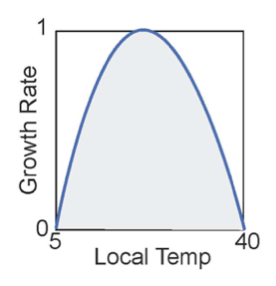
In this model, the death rate, D, is just a constant, but the growth rates depend on the temperature.  The idea here is that there is an optimum temperature for growth (22.5°C) and a temperature range where growth can occur (between 5° and 40°C).  We will make the assumption that the relationship between the temperature and the growth rate has the form of a parabola, expressed in the following equations:

Tw and Tb refer to the temperatures of the white and

black areas — they differ from each other and from the

average planetary temperature because of their albedos. 

These local temperatures are given by the following:

Here, fHA is the heat absorption factor (a constant value — 20), α is the albedo (subscripts refer to white areas, black areas, and the planetary average, and Tp is the average planetary temperature.  As a consequence of the value for fHA and the specified albedos, Tw will be 5° C cooler than the planetary average if the planetary albedo is 0.5; black areas will have a local temperature 5° C warmer than the average.

The average planetary albedo in the above equation is a function of the areas covered by the daisies and the specified albedos, as described in the following:

The final part of the model is the calculation of the planetary temperature.  For this, we will use a simple formulation for the equilibrium temperature based on the assumption that the energy absorbed from the sun is equal to the energy emitted by the planet:

The energy absorbed is a function of the energy intensity of sunlight and the planetary albedo, expressed here as:

S is something called the solar flux constant, set by Watson and Lovelock to be 917 W/m2, while L is called the luminosity factor, which varies from 0.6 to 1.8 over the lifespan of Daisyworld (assumed to be 2 billion years).  So, Daisyworld is like the Earth in the sense that its sun emits more energy over the lifetime of the planet.  The energy emitted comes from the simple blackbody radiation law:

Here, σ is the Stefan-Boltzmann constant, which is 5.67 x 10-8 Wm-2K-4.  Combining these two equations, we have:

This can be rearranged to give the temperature (in °C) of the planet:

Together, these equations form the basis of the Daisyworld model we will work with in STELLA.

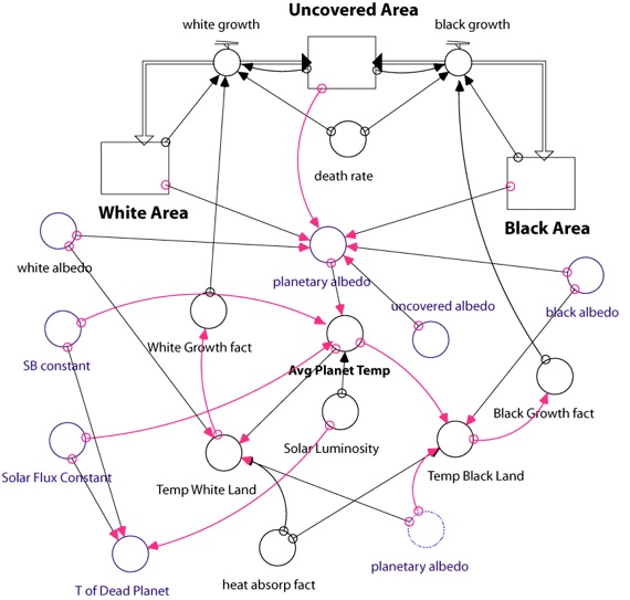
Here is the STELLA diagram for the construction of this system.  Note that the reservoirs represent area, or really, the fraction of the total area covered by the daisies or empty (uncovered).  First, build this model using the equations below, and then we’ll do some experiments.

Equations for Daisyworld Model

Reservoirs: (make sure these are all non-negative by clicking the appropriate box)

INIT Uncovered_Area = 1.0 {portion of surface that daisies can occupy}

INIT Black_Area = 0

INIT White_Area = 0

 

Flows: (make sure these are defined as biflows)

black_growth = Black_Area*(Uncovered_Area*Black_Growth_fact - death_rate)+.001

{the .001 is needed to give the system a bit of a nudge; without it the daisies never get                     going}

white_growth = White_Area*(Uncovered_Area*White_Growth_fact - death_rate)+.001

{the .001 is needed to give the system a bit of a nudge; without it the daisies never get going}

 

Converters:

death_rate = 0.3

uncovered_albedo = .5

white_albedo = .75

black_albedo = .25

Black_Growth_fact = 1 -.003265*((22.5 - Temp_Black_Land)^2) {equation for a parabola}

White_Growth_fact = 1 - .003265*((22.5-Temp_White_Land)^2) {equation for a parabola}

Temp_Black_Land = heat_absorp_fact*(planetary_albedo - black_albedo)+Avg_Planet_Temp

Temp_White_Land = heat_absorp_fact*(planetary_albedo - white_albedo)+Avg_Planet_Temp

heat_absorp_fact = 20 {this controls how the local temperatures of the daisies differ from the average planetary temperature}

planetary_albedo = (Uncovered_Area*uncovered_albedo)+(Black_Area*black_albedo)+(White_Area*white_albedo)

Solar_Flux_Constant = 917 { Wm-2  -- for reference, our Sun cranks out 1370 Wm-2 }

SB_constant = 5.67E-8 {Stefan-Boltzmann constant Wm-2T-4}

Solar_Luminosity = 0.6+(time*(1.2/200)) {this makes a straight line going from .6 to 1.8 over 200 time units; each time unit is 10 million years}

Avg_Planet_Temp = ((Solar_Luminosity*Solar_Flux_Constant*(1-planetary_albedo)/SB_constant)^.25)-273 {energy balance to calculate temperature in °C}

T_Dead_Planet = ((Solar_Luminosity*Solar_Flux_Constant*(1 - .5)/SB_constant)^.25)-273 {energy balance to calculate temperature in °C of a planet with no daisies}

 Run Specs:

0 to 200  (one time unit = 10 million years)

Time step = 0.25

Integration: Runge-Kutta 4