Constraints on Population Growth

Modeling the Future of Food, Soil, and Population
In this module, we will explore the connections between human population growth and food production, which includes soil as a resource that influences how much food we can produce. Food is obviously a huge concern for the future. Most estimates indicate that we will have 9 billion people by 2050 — that is 2 billion more mouths to feed than today. It is likely that the demand for food will go up even more; if economic development continues its recent trend and people become wealthier, they will desire richer diets with more meat, and that means that we may have to double our current food production to meet these demands. Of course, these demands may not be met and people will have to settle for a leaner diet. This is obviously an issue that deserves a close look, and we'll do this usng a set of STELLA models in this lab activity.
Simple Population Growth
To begin with, let’s try to understand a few basic things about population growth by exploring a very simple model of the global population. The model looks like this:
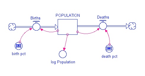
Population starts out with 7 billion people; it increases due to births and decreases due to deaths — what could be simpler? The birth percent is a constant and gets multiplied by the population to give the number of people born each year; likewise, the death rate is also constant and is multiplied by the population to give the number of people who die each year. Log Population is just a converter that gives the logarithm of the population, which is sometimes a useful thing to look at when studying population growth (remember that log(10) =1, log(100)=2, log(1000)=3, etc.). Sometimes population growth follows an exponential curve, and the log of an exponential curve is a straight line.
The initial birth percent at present is about 1.91% per year, while the death percent is about 0.88%, so the net growth rate is 1.03% per year — more people are born each year than die each year, and thus our population grows.
Let’s do a couple of experiments with this model to get a better feel for population growth.
1. Run the model and observe what happens. Note that the Population itself is an exponential curve (slope keeps getting steeper and steeper), while the log of the population is a straight line that could be extrapolated out into the future to predict the population. From the model, what is the population in the year 2200?
2. Look on graph 3 and describe the difference between births and deaths as time goes on.
3. Now make the birth percent .01 (1%) and the death percent .02 (2%) and observe what happens. What is the population by the year 2200?
Constraints on Population Growth
Your answer to question 1 above should strike you as absurd — the Earth surely cannot support that many people. This means that there are some natural constraints on the size of the population, and one of those constraints is food. But another could be something like diseases that become much more effective as the population becomes very crowded. Another constraint might be pollution, as represented in the model diagram below:
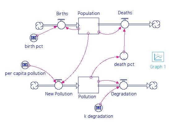
Here, we see another reservoir called Pollution that increases due to human activities that create pollution; this is controlled by a per capita pollution value. The pollution is degraded (altered, broken down, and rendered harmless) according to a rate constant. The amount of pollution influences the death percent of the population — as pollution goes up, so does the death percent. So, the basic ideas here are pretty simple but not too realistic since the death percent may be a function of many different factors. Nevertheless, we will do a couple of experiments with this model just to see what the implications of these connections are in terms of the population growth.
4. Run the model as it is set up and describe what happens to the Population and Pollution reservoirs. The units of population are billions of people, and the units of pollution are some unspecified global mass of pollution. Take note of the maximum population that is attained in this model.
5. Now try increasing the per capita pollution from 0.5 to 1.0, run the model and compare the maximum population to that of the initial model. Then decrease it to 0.25, run the model again and take note of the maximum population. What is the relationship between the per capita pollution and the maximum population?
6. Now do a similar experiment with the degradation rate constant — first increase it to 0.1 and then decrease it to 0.025, and take note of the maximum population and the character of the oscillation. What is the relationship between this degradation rate constant and the maximum population and the nature of the oscillation?
An aside on oscillations… This very simple model we just examined has a tendency to oscillate under certain conditions, and as it turns out, this is a fairly common kind of behavior when you have systems in which there are two or more entities that affect each other. A well-known example is the populations of rabbits and lynxes in Canada — these species are closely interconnected and their populations tend to oscillate over time. ENSO is another example of an oscillation in which the winds and the sea surface temperatures interact with one another to cause an oscillation in the warm water pool in the equatorial Pacific.
Population and Food
Now we turn to some models where food provides a constraint on population growth — just as Malthus suggested long before the age of computers. This model is also pretty simple, but it will allow us to explore the possible consequences of the future of food production as predicted by the Food and Agriculture Organization of the United Nations (FAO). The FAO notes that in recent times, global food production has increased at an annual rate of about 2% per year, but this rate of increase has been declining over time and they expect it to continue that trend in the future. The reason for this is that as we have increased agricultural yields from the land, we have approached a sort of maximum value that is possible, and as we approach that limit, it gets harder and harder to make the same gains in food production that we have obtained in the past.
Here is what the model looks like:
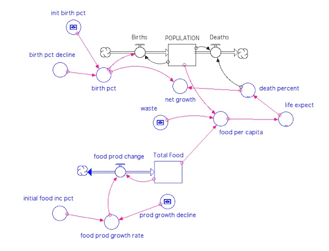
In this model, the amount of food produced each year determines the amount of food per capita, and that affects the life expectancy, which in turn affects the death rate. Total Food represents the food produced each year, and it assumes that all of this is consumed that year; it increases following a food production growth rate that is essentially the percent per year by which our food production increases. This growth rate, as mentioned above, declines according to a parameter called the production growth decline. The model also includes waste — it turns out that at present, almost 30% of the food we produce is wasted due to the imperfect distribution of food to places where it is needed. The model is initially set up with a production growth decline factor of 2% per year.
This model also includes something that will decrease the global birth percent per year, following the best estimates of demographers — this will limit the rate at which the population increases.
7. Run the model with all of the parameters in their initial states (i.e., don’t change anything) and observe what happens. The population levels off at about 25 billion by the year 2400, and it gives us something close to the expected 9 billion by the middle of this century. This leveling off, or approach to steady state, means that the birth and death percents must be just about equal, but at the beginning, the birth percent is certainly higher than the death percent since the population increases. The question here is: How does the food production history contribute to the leveling off of the population? Study the Total Food reservoir, the food per capita, the life expectancy, and the death percent as you search for an answer.
8. What if we eliminate waste? Change the waste value from 0.3 to 0.0 and run the model, comparing the results to the initial model with waste set at 0.3.
9. Restore all the parameters to their beginning values, and then change the production growth decline from 0.02 (this is 2%) to 0.0. This is like saying that we will somehow be able to continue our increasing rate of food production indefinitely — a very optimistic outlook. Run the model and describe what happens in terms of the ending population, the general form of the population curve, and the food per capita.
10. Next, change the production growth decline from 0.02 to 0.04, which is like saying that our ability to increase food production will diminish even faster than the FAO predicts. Run the model and describe what happens in terms of the ending population, the general form of the population curve, and the food per capita.
Population, Food, and Soil
Note that in the above models, the Total Food always increases, or in the worst case, it levels off to a constant value. But is this realistic? Where does food come from in the first place? Answer: the soil.
Is soil a limitless resource? No, it is not; if soils are eroded, you cannot grow crops on the underlying rock and we cannot transform that rock magically to soil.
Is soil a renewable resource? Yes, it is renewed in the sense that there are natural processes (chemical weathering of rocks and biological alteration of the weathered material) that create soils. But these processes are slow, so that if global erosion of soils exceeds the natural formation of soils, then global soils are a diminishing resource and our ability to produce food from this diminishing resource will make it even more challenging to meet the food demands of the future.
How much soil is lost to erosion each year? This is not an easy thing to measure, but it is important, and lots of scientists have studied this; the result is an estimate of about 35 GT of soil per year, which is about 1% of the global stock of soil in farmable regions (3500 GT). Soil erosion is highly variable across the globe, and in some areas (the US, for example) soil erosion has been reduced, but in many other areas in developing nations, it is on the rise. In the effort to produce more and more food, people tend to ignore farming practices that could minimize soil erosion.
So how fast is soil formed? This is also a tough thing to measure, but on a global basis, it would appear to be somewhere around 7 GT of new soil formed per year (this gives a residence time for soil of about 500 years, which agrees with average radiocarbon dates of soils). So, we are losing more soil than we are gaining, which is not a good thing for the future of food production and population.
Let’s explore this a bit more by using another model, one in which the food production that is achieved is partly related to technological advances in farming, and partly related to how much soil there is. Here is the model:
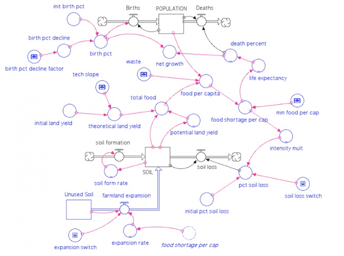
You can see that this is now a bit more complicated, but the population part of the model is the same as before — it is set up to run from the present to 400 from now and the birth rate declines as before (you can adjust how much it declines in this case), while the death percent is controlled by the life expectancy, which is connected to food per capita (really the food shortage per capita, which might be a more flexible measure of nutrition).
There are a few critical things to understand about this model, in addition to the basic fact that at the start, we are losing more soil than is being produced.
The total food available each year is related to what kind of yield is possible given technological advances and given what the soil will allow as an upper limit. Technology here advances at a constant 2% per year, which is optimistic, but not ridiculous. The upper limit that the soil will allow in terms of calories of food per ton of soil depends on how much soil there is. As the amount of soil drops this upper limit gradually decreases, but the decrease becomes quite dramatic as the soil vanishes. If the technologically possible yield is greater than what the soil will allow, then the soil’s limit determines how much food is produced, but if the technologically possible yield is less than what the soil will allow, then technology’s limit determines how much food is produced.
The model includes something called the food shortage per capita, which depends on the food per capita and a perception of what the minimum acceptable value is. The minimum food per capita is initially set to be 3000 kilocalories per person per day (I know this seems like a lot, but this is really all of the food energy that goes into producing the couple of thousand of calories we take into our mouths each day — the process of getting things from the soil and into our mouths is obviously quite inefficient!). Note that if this is a negative value, it is really a food surplus per capita. The minimum food per capita can be adjusted up or down; if it moves down, that is like saying that we become more efficient in bringing food to the table. One way to do this is by eating less meat. since converting grain into meat involves a loss of energy. Eating less meat, or meat that is produced more efficiently. doesn’t mean that we would all have to become vegetarians, it might just mean that we scale back our meat consumption.
This food shortage per capita can then trigger some responses that impact the soil part of the model. As the food shortage become more acute, one possibility is that people will try to farm more intensively, which tends to increase soil erosion; on the other hand, a food surplus might lead to less intensive farming, thus slowing soil erosion. The food shortage per capita connects to soil erosion through something called the intensity multiplier, which is multiplied by the starting rate of soil erosion. This effect can be turned on or off with a switch.
The food shortage per capita is also connected to another part of the model representing the expansion of farmland. The model assumes that there is something like 20% more farmable land to be utilized (this is a generous assumption) and as the food shortages become acute, there will obviously be incentives to farm this land. In the model, this is a flow of new soil into the soil reservoir that is then available for food production. This too can be turned on or off with a switch.
The soil formation is set up so that it increases as the soil is depleted; if all the soil is removed, then the rate of formation is 50 GT per year rather than the present day value of 7 GT per year.
Now that you know a few of the basics of this model, let’s try a few things with it. A model like this could keep you busy for a long time, changing everything, but we’ll just alter a few basics things here.
11. Run the model with the parameters set to their starting condition and see what happens, then describe what the population does — does it rise and stabilize at some high level (If so, at what value?), or does it peak (If so, what is the peak value, and when does it occur?) and then collapse to zero, or does it peak and collapse to some lower level (If so, what is the population at that more or less stable point?).
12. How does this history change if we eliminate waste?
13. What if we turn off the soil loss switch? This is like saying that even if food shortages become acute, we will not do anything to worsen the erosion of soil. In this way, the starting rate of soil loss in terms of a percentage will remain constant. Before doing this, remember to return the waste parameter to its initial value of 0.3. As before, describe the pattern of the population curve.
14. Now let’s see if we can find a more sustainable path for the population. Try different combinations of the soil loss switch on or off, the farmland expansion switch on or off, waste higher or lower, the birth rate decline factor higher or lower, and the minimum food per capita higher or lower. Reducing the minimum food per capita is like saying that we find a way to feed ourselves more efficiently. Your goal is to find the combination of these parameters that lead to a population history that comes the closest to rising and then leveling off without a drastic reduction (which would probably be unpleasant), with the lowest possible food shortage per capita (negative is better here). Remember that the goal is not just to have the largest population.
Hopefully, you see that although we are not on a sustainable path at present, there are some ways that we can alter our situation and come to a more sustainable future while avoiding a large population crash that might be accompanied by good deal of conflict and misery.