Experiment 1: The First Run

What will happen to the temperature of the Earth if we run the model for 30 years with the following initial conditions:

Initial Temp = 0°C

Albedo = 0.3    (this will not change over time)

Emissivity = 1.0    (this will not change over time)

Ocean Depth = 100 m    (this will not change over time)

Solar Constant = 1370 W/m2   To set this, double-click on the icon and you will see a graph of the Solar Constant vs Time, along with 2 columns on the right.  If you are running the model in STELLA, you should see a window like this:

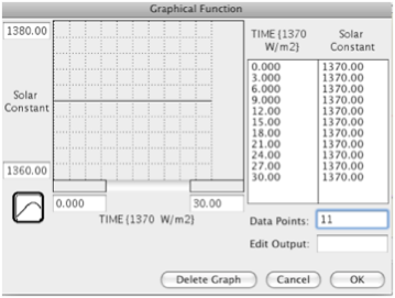
You can alter the value of the Solar Constant by changing the values in the column on the right, or by clicking at different grid points on the graph.  The Solar Constant should be set up as a straight line when you first open the model.

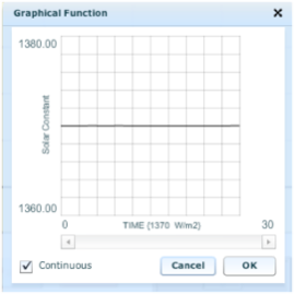
If you are running the model on the web, you should see a window like this:

Before running the model, stop to think about the inflows and the outflows.  The solar constant, the albedo, and the cross-sectional area will not change over time in this model, so the energy in, the Insolation, will be constant.  How about the energy flowing out — will it remain constant?  Some of the model components feeding into this flow are constants during the model run; the emissivity, the Stefan-Boltzmann constant, the surface area of the Earth.  But, the temperature may change if the amount of energy stored in the reservoir changes.  If there is more energy coming in that leaving at the beginning of the model, then the temperature will rise; if the temperature rises, then the amount of energy emitted goes up.  Will it continue to go up forever?

Let’s try to make a careful estimate of what things will look like at the very start of this model’s run.  The Insolation is:

1370 ∗ (πR2) ∗ (1-α) ∗ 3.15e7  [J/yr],   (3.15e7 s/yr)

which gives an initial value of about 3.8e24 [J/yr].  Now compare this to the Heat Emitted:

(4πR2) ∗ 1 ∗ 5.67e-8 ∗ T4 ∗ 3.15e7  [J/yr], (5.67e-8 is the S-B constant, 1 is the emissivity, T is 273 °K)

which results in a value of  about 5e24 [J/yr] — greater than the value of the Insolation. 

So our planet is losing more energy than it gains — thus the temperature must decrease.

1a.  If the temperature decreases as we move one step forward in time, what happens to the amount of Heat Emitted in that next step?  Does it increase, decrease, or stay the same? Explain your reasoning (think about the Stefan-Boltzman Law).

Experiment 1  The Initial Run

1b. Now try to imagine what will happen after many steps through time. Illustrate your thinking by drawing curves on the graphs below that chart Insolation, Heat Emitted, and Temperature over time.

1c. Now run the model and see what happens.  Look at the Insolation over time — does it change or remain the same?  Was your prediction good or bad?

1d. Look at the Heat Emitted over time — does it change or remain the same?  Did you predict this pattern, or does it surprise you?

1e. Describe how the temperature changes — where does it start, what is it at the end, how does it change in the time between?  Is the change steady, making a straight line, or is it curved?  Write your answer below.

1f. What is the temperature at the end of the 30 years?

Time

Time

Time

Experiment 2 — Finding the Steady State

2a.  Now, let’s change the initial temperature from 0°C to 40°C.  Keep everything else the same.  Run the model and watch the temperature.  Now, change the initial temperature to 20°C and run it again.  Then, change the initial temperature to -20°C and run it again.  Where does the temperature end up in each case?

2b. Steady state for a system is the condition in which the system components are not changing over time even though time is running and things are moving through the system. What is the steady state temperature of this system?

3a. Next, let’s try to do something about the dismal steady state temperature of our system — it is way too cold for my taste!  And, it does not reflect what our global average temperature actually is — about 15°C.  What we have not included here, at least by name, is the effect of the heat-trapping gases in our atmosphere, a.k.a., the greenhouse effect.  As you should recall from the background reading, these gases trap heat emitted by the surface and then send a good portion of that heat back down to the surface — this means that the heat actually emitted into outer space is considerably less than it should be.  In the model, this effect is represented by the emissivity.  When the emissivity is 1.0, then the planet emits energy like a perfect blackbody — not too realistic. Set the following initial conditions:

Initial Temp = 0°C

Albedo = 0.3    (this will not change over time)

Solar Constant = 1370 W/m2   (this will not change over time)

Emissivity = 0.6147    (this will not change over time)

Ocean Depth = 100 m    (this will not change over time)

Run the model two more times with different initial temperatures.  Does the model converge on a single steady state temperature?  If so, what is that temperature?

3b. In general, how do you predict the steady state temperature will change if the emissivity decreases to something like 0.5?  Will the steady state temperature be warmer or colder than the last experiment, with ε=.6147?  Explain your reasoning.

Experiment 3 — Warming the Planet

We think that at several times in Earth’s past, it was almost completely covered in ice — the Snowball Earth condition.  One way to represent this is to have the albedo of the planet increase to a value that would represent most of the surface covered by snow and ice (0.9) and clouds (.5 to .6). We’ll choose a planetary albedo of 0.7.  Set the model up with the following parameters:

Initial Temp = 15°C

Albedo = 0.7   

Solar Constant = 1370 W/m2  

Emissivity = 0.6147   

Ocean Depth = 100 m   

4a.  Make a prediction about what you think will happen to the temperature?

4b. Run the model and find the steady-state temperature of the planet.

4c. What would life be like on a planet like this? Pleasant or unpleasant?

Experiment 4 — An Ice-covered Planet

Experiment 5 — A Variable Sun

The Solar Constant is not really constant over any length of time.  For instance, it was only 70% as bright early in Earth’s history, and it undergoes much more rapid fluctuations (but much smaller) in association with the 11 year sunspot cycle.  During a sunspot cycle, the solar constant may vary by as much as 4 W/m2.  Let’s see what this would do to the temperature of the planet.  Set the model up with the following parameters:

Initial Temp = 15°C

Albedo = 0.3   

Emissivity = 0.6147   

Ocean Depth = 100 m

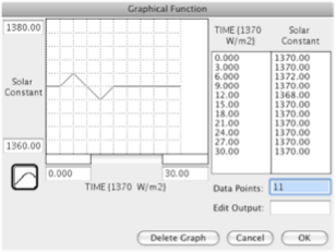
Solar Constant  — a graphical function of time as shown at right:

This will create an increase of 2 W/m2 and then a decrease of 2 W/m2 in the Solar Constant over a period of 12 years — a pretty good approximation of a solar sunspot cycle.

5a. Run the model and see what happens.  How much does the planetary temperature change over the solar cycle (difference between peak and trough)?

5b.  Notice that the temperature peaks after the Solar Constant peaks.  This time delay is called a lag time.  What is the lag time here?

5c. Predict how the model will change is you increase the ocean depth to 200 m.  Comment on the lag time and the magnitude of temperature change relative to the first solar cycle model (6a).

5d. Now run the model.  Compare the model results with your predictions.

5e. Did the model have time to fully adjust to the increase (or decrease) in the Solar Constant?  Let’s investigate this by modifying the Solar Constant graph so that it starts at 1370, and then jumps up quickly to 1372 and then stays there for the rest of the model time.   Compare the rise in temperature to the rise seen in experiment 6a (take half of your answer from 6a), and then say whether the system had time to fully adjust to the increased solar input during experiment 6a.