The following article by Dr Marsha Singh, Queen's University Physics Department, is verbatim from:

http://physics.queensu.ca/~marsha/SAXSoverview.html    

A Brief  Overview of SAXS

     Small angle x-ray scattering (SAXS) is a very well-established measurement  tool that has been around for about 70 years. It is "special"  in terms of the distinction between SAXS and regular wide-angle x-ray  scattering by virtue of the location of the scattering of interest. This  is typically at small angles in the vicinity of the primary beam and  extending to less than 2 degrees for standard wavelengths. The scattering features at these angles correspond to structures ranging from tens to  thousands of angstroms.

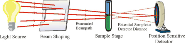
Figure 1:  Schematic SAXS Apparatus

Why SAXS?

     Why do SAXS, instead of, say light scattering or electron microscopy which  might be considerably more straightforward? In many cases, we need to  look at bulk materials which are opaque to visible light. The need to  produce very thin slices for electron microscopy can destroy the very  thing we want to look at. Small angle neutron scattering is usually a  possibility but certainly no more straightforward than SAXS. In the cases  described in this document, SAXS is either the best or the only source of  the information that we needed on our materials.

 How can SAXS be  performed?

     The primary experimental ingredients to SAXS is  the need for a well-collimated x-ray beam with a small cross-section.  Synchrotron radiation sources with their intense brightness and natural  collimation are ideal when we consider the fact that most polymer  materials are very poor scatterers.

     There is always some form of beam shaping required to  maintain the small cross-section in going from the source to the sample  and to reduce distortions from parasitic scattering from whatever  obstacles, including air, are encountered. This is where much of the  experimental effort is required. A sample stage that may or may not involve heating elements, tensile stress apparatus, etc., then follows,  ideally all within an in-vacuum path. No preparation such as staining of  the material is required, and thicknesses of between 1 and 3 mm are  usually fine. As shown here, and indeed in most  typical experiments, the SAXS technique is performed in transmission  mode. In this mode, polymer samples are typically 1-2mm thick, offering  about 63% absorbtion of the incident x-ray  beam.

     In situations where transimission  mode operation is not a feasable option, such  as when the sample of interest is a thin film on an opaque substrate of  when only the surface microstructure is of interest, one must resort to  using a combination of Grazing Incidence Diffraction geometry and SAXS,  known as GISAXS.  More information about GISAXS is available at the link provided.

     An extended sample-detector distance is usually  required to give the barely scattered photons room to spread out from the  main beam and also to reduce the detected x-ray background. Finally, a  position sensitive detector, ideally 2-dimensional, is required to  measure the scattered intensity. As sketched here, the black spot would  be the beamstop that is absolutely essential to  block the main beam and the rings are a cartoon of the Debye rings one would see from an ordered structure.  As we will see, most SAXS data is much less straightforward and appears as a continuous function of scattering angle. For analysis, we will  usually have to reduce this 2-D profile to a 1-D set of intensity vs.  angle data.

 SAXS Data Analysis

     Interpreting SAXS data can be a very difficult task unless one is very  lucky and the sample fits one of the many idealized models that have been  developed over the years. Regular WAXS tends to focus on the location,  width, shifts, etc. of Bragg peaks which arise from crystalline lattice structures.  One can still observe Bragg peaks in SAXS but these will result from  regular spacings that are on the order of hundreds of Angstroms. Most of the time, however, the observed curves  tend to be apparently featureless.

     At very small angles, the shape of the scattering in  the so-called Guinier region can be used to  give us an idea of the radius of gyration of any distinct structures that  are on this type of lengthscale.

     At higher angles, if we had a system of relatively  identical particles, dilute enough for there to be no interactions, we  might be able to see broad peaks that would also give us information on  the shape of the particles. The sketch here showing Bragg peaks  corresponds to a system of strongly interacting particles which would obscure this type of single-particle information.

     At still higher angles, the so-called Porod region, the shape of the curve is useful in obtaining information on the surface-to-volume ratio of the scattering  objects. This can also be used to can information on the dimensions of  our scattering particles.

     Finally, the area under the curve gives us the  so-called INVARIANT which is a measure of how much scattering material is  seen by our beam. Changes in the invariant are useful in monitoring the  crystallization process in polymer materials.

     All of these are so-called DIRECT methods of analysis  which give us information based on interpretation of the clean  (background corrected) data with no further manipulation. However, all of  these parameters are based on well-defined assumptions such as the  existence of uniform density within our so-called particle, uniform  density in the background, sharp interfaces between the two, etc. We can  go further when these approximations do not apply by fourier  transforming the data to get real space information (such as obtainable  by electron microscopy). We've used the GNOM routine provided by a  Russian colleague for this purpose.

     We can also propose specific structures, calculate the  scattering, then fit the data to obtain the  parameters defining our model structure. This tends to imply that we already know the answer, not the general case.

     Finally, when we don't really have any clear order to  base our interpretation on, we can assume a strongly DISORDERED structure  and turn to fractal analysis (where the disorder is itself a form of  order) or paracrystal analysis (where the  system is really just a heavily distorted regular structure).

 Further Reading

·   M.A. Singh and C. Barberato, Small-Angle X-ray Scattering from  Soft Materials, Physics in Canada,  September/October 1997.

·   O. Glatter  and O. Kratky, Small Angle X-ray  Scattering, New York:  Academic Press, 1982.

·   L.A. Feigin  and D.I. Svergun, Structure Analysis by  Small-Angle X-ray and Neutron Scattering, New York: Plenum Press, 1987.